📊Graphical Representation: Graphics We Live By (Part VIII: List of Items in Power BI)

Graphical Representation Series

Introduction

There are situations in which one needs to visualize only the rating, other values, or ranking of a list of items (e.g. shopping cart, survey items) on a scale (e.g. 1 to 100, 1 to 10) for a given dimension (e.g. country, department). Besides tables, in Power BI there are 3 main visuals that can be used for this purpose: the clustered bar chart, the line chart (aka line graph), respectively the slopegraph:

Main Display Methods

Main Display Methods

For a small list of items and dimension values probably the best choice would be to use a clustered bar chart (see A). If the chart is big enough, one can display also the values as above. However, the more items in the list, respectively values in the dimension, the more space is needed. One can maybe focus then only on a subset of items from the list (e.g. by grouping several items under a category), respectively choose which dimension values to consider. Another important downside of this method is that one needs to remember the color encodings. 

This downside applies also to the next method - the use of a line chart (see B) with categorical data, however applying labels to each line simplifies its navigation and decoding. With line charts the audience can directly see the order of the items, the local and general trends. Moreover, a line chart can better scale with the number of items and dimension values.

The third option (see C), the slopegraph, looks like a line chart though it focuses only on two dimension values (points) and categorizes the line as "down" (downward slope), "neutral" (no change) and "up" (upward slope). For this purpose, one can use parameters fields with measures. Unfortunately, the slopegraph implementation is pretty basic and the labels overlap which makes the graph more difficult to read. Probably, with the new set of changes planned by Microsoft, the use of conditional formatting of lines would allow to implement slope graphs with line charts, creating thus a mix between (B) and (C).

This is one of the cases in which the Y-axis (see B and C) could be broken and start with the meaningful values. 

Table Based Displays

Especially when combined with color encodings (see C & G) to create heatmap-like displays or sparklines (see E), tables can provide an alternative navigation of the same data. The color encodings allow to identify the areas of focus (low, average, or high values), while the sparklines allow to show inline the trends. Ideally, it should be possible to combine the two displays.  

Table Displays and the Aster Plot

One can vary the use of tables. For example, one can display only the deviations from one of the data series (see F), where the values for the other countries are based on AUS. In (G), with the help of visual calculations one can also display values' ranking. 

Pie Charts

Pie charts and their variations appear nowadays almost everywhere. The Aster plot is a variation of the pie charts in which the values are encoded in the height of the pieces. This method was considered because the data used above were encoded in 4 similar plots. Unfortunately, the settings available in Power BI are quite basic - it's not possible to use gradient colors or link the labels as below:

Source Data as Aster Plots

Sankey Diagram

A Sankey diagram is a data visualization method that emphasizes the flow or change from one state (the source) to another (the destination). In theory it could be used to map the items to the dimensions and encode the values in the width of the lines (see I). Unfortunately, the diagram becomes challenging to read because all the lines and most of the labels intersect. Probably this could be solved with more flexible formatting and a rework of the algorithm used for the display of the labels (e.g. align the labels for AUS to the left, while the ones for CAN to the right).

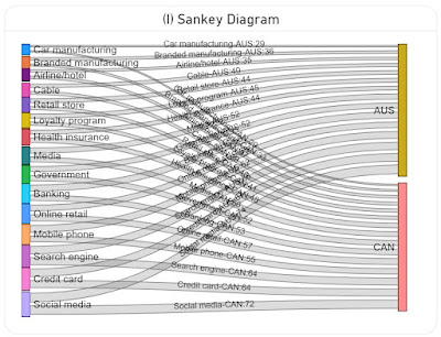
Sankey Diagram

Data Preparation

A variation of the above image with the Aster Plots which contains only the plots was used in ChatGPT to generate the basis data as a table via the following prompts:

• retrieve the labels from the four charts by country and value in a table
• consolidate the values in a matrix table by label country and value

The first step generated 4 tables, which were consolidated in a matrix table in the second step. Frankly, the data generated in the first step should have been enough because using the matrix table required an additional step in DAX.

Here is the data imported in Power BI as the Industries query:

let
    Source = #table({"Label","Australia","Canada","U.S.","Japan"}
, {
 {"Credit card","67","64","66","68"}
, {"Online retail","55","57","48","53"}
, {"Banking","58","53","57","48"}
, {"Mobile phone","62","55","44","48"}
, {"Social media","74","72","62","47"}
, {"Search engine","66","64","56","42"}
, {"Government","52","52","58","39"}
, {"Health insurance","44","48","50","36"}
, {"Media","52","50","39","23"}
, {"Retail store","44","40","33","23"}
, {"Car manufacturing","29","29","26","20"}
, {"Airline/hotel","35","37","29","16"}
, {"Branded manufacturing","36","33","25","16"}
, {"Loyalty program","45","41","32","12"}
, {"Cable","40","39","29","9"}
}
),
    #"Changed Types" = Table.TransformColumnTypes(Source,{{"Australia", Int64.Type}, {"Canada", Int64.Type}, {"U.S.", Number.Type}, {"Japan", Number.Type}})
in
    #"Changed Types"

Transforming (unpivoting) the matrix to a table with the values by country:

IndustriesT = UNION (
    SUMMARIZECOLUMNS(
     Industries[Label]
     , Industries[Australia]
     , "Country", "Australia"
    )
    , SUMMARIZECOLUMNS(
     Industries[Label]
     , Industries[Canada]
     , "Country", "Canada"
    )
    , SUMMARIZECOLUMNS(
     Industries[Label]
     , Industries[U.S.]
     , "Country", "U.S."
    )
    ,  SUMMARIZECOLUMNS(
     Industries[Label]
     , Industries[Japan]
     , "Country", "Japan"
    )
)

Notes:

The slopechart from MAQ Software requires several R language libraries to be installed (see how to install the R language and optionally the RStudio). Run the following scripts, then reopen Power BI Desktop and enable running visual's scripts.

install.packages("XML")
install.packages("htmlwidgets")
install.packages("ggplot2")
install.packages("plotly")

Happy (de)coding!

Previous Post <<||>> Next Post

📊Graphical Representation: Graphics We Live By (Part VI: Conversion Rates in Power BI)

Graphical Representation Series

Introduction

Conversion rates record the percentage of users, customers and other entities who completed a desired action within a set of steps, typically as part of a process. Conversion rates are a way to evaluate the performance of digital marketing processes in respect to marketing campaigns, website traffic and other similar actions. 

In data visualizations the conversion rates can be displayed occasionally alone over a time unit (e.g. months, weeks, quarters), though they make sense only in the context of some numbers that reveal the magnitude, either the conversions or the total number of users (as one value can be calculated then based on the other). Thus, it is needed to display two data series with different scales if one considers the conversion rates, respectively display the conversions and the total number of users on the same scale. 

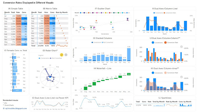
For the first approach, one can use (1) a table or heatmap, if the number of values is small (see A, B) or the data can be easily aggregated (see L); (2) a visual with dual axis where the values are displayed as columns, lines or even areas (see E, I, J, K); (3) two different visuals where the X axis represents the time unit (see H); (4) a visual that can handle by default data series with different axis - a scatter chart (see F). For the second approach, one has a wider set of display methods (see C, D, G), though there are other challenges involved.

Conversion Rates in Power BI

Tables/Heatmaps

When the number of values is small, as in the current case, a table with the unaltered values can occasionally be the best approach in terms of clarity, understandability, explicitness, or economy of space. The table can display additional statistics including ranking or moving averages. Moreover, the values contained can be represented as colors or color saturation, with different smooth color gradients for each important column, which allows to easily identify high/low values, respectively values from the same row with different orders of magnitude (see the values for September).

In Power BI, a simple table (see A) allows to display the values as they are, though it doesn't allow to display totals. Conversely, a matrix table (see B) allows to display the totals, though one needs to use measures to calculate the values, and to use sparklines, even if in this case the values displayed are meaningless except the totals. Probably, a better approach would be to display the totals with sparklines in an additional table (see L), which is based on a matrix table. Sparklines better use the space and can be represented inline in tables, though each sparkline follows its own scale of values (which can be advantageous or disadvantageous upon case).

Column/Bar Charts 

Column or bar charts are usually the easiest way to encode values as they represent magnitude by their length and are thus easy to decode. To use a single axis one is forced to use the conversions against the totals, and this may work in many cases. Unfortunately, in this case the number of conversions is small compared with the number of "actions", which makes it challenging to make inferences on conversion rates' approximate values. Independently of this, it's probably a good idea to show a visual with the conversion rates anyway (or use dual axes).

In Power BI, besides the standard column/bar chart visuals (see G), one can use also the Tornado visual from Microsoft (see C), which needs to be added manually and is less customizable than the former. It allows to display two data series in mirror and is thus more appropriate for bipartite data (e.g. males vs females), though it allows to display the data labels clearly for both series, and thus more convenient in certain cases. 

Dual Axes 

A dual-axis chart is usually used to represent the relationship between two variables with different amplitude or scale, encoding more information in a smaller place than two separate visuals would do. The primary disadvantage of such representations is that they take more time and effort to decode, not all users being accustomed with them. However, once the audience is used to interpreting such charts, they can prove to be very useful.

One can use columns/bars, lines and even areas to encode the values, though the standard visuals might not support all the combinations. Power BI provides dual axis support for the line chart, the area chart, the line and staked/clustered column charts (see I), respectively the Power KPI chart (see E). Alternatively, custom visuals from ZoomCharts and other similar vendors could offer more flexibility.  For example, ZoomCharts's Drill Down Combo PRO allows to mix  columns/bars, lines, and areas with or without smooth lines (see J, K).

Currently, Power BI standard visuals don't allow column/bar charts on both axes concomitantly. In general, using the same encoding on both sides of the axes might not be a good idea because audience's tendency is to compare the values on the same axis as the encoding looks the same. For example, if the values on both sides are encoded as column lengths (see J), the audience may start comparing the length without considering that the scales are different. One needs to translate first the scale equivalence (e.g. 1:3) and might be a good idea to reflect this (e.g. in subtitle or annotation). Therefore, the combination column and line (see I) or column and area (see K) might work better. In the end, the choice depends on the audience or one's feeling what may work. 

Radar Chart

Radar charts are seldom an ideal solution for visualizing data, though they can be used occasionally for displaying categorical-like data, in this case monthly based data series. The main advantage of radar charts is that they allow to compare areas overlapping of two or more series when their overlap is not too cluttered. Encoding values as areas is in general not recommended, as areas are more difficult to decode, though in this case the area is a secondary outcome which allows upon case some comparisons.

Scatter Chart

Scatter charts (and bubble charts) allow by design to represent the relationship between two variables with different amplitude or scale, while allowing to infer further information - the type of relationship, respectively how strong the relationship between the variables is. However, each month needs to be considered here as a category, which makes color decoding more challenging, though labels can facilitate the process, even if they might overlap. 

Using Distinct Visuals

As soon as one uses distinct visuals to represent each data series, the power of comparison decreases based on the appropriateness of the visuals used. Conversely, one can use the most appropriate visual for each data series. For example, a waterfall chart can be used for conversions, and a line chart for conversion rates (see H). When the time axis scales similarly across both charts, one can remove it.

The Data

The data comes from a chart with dual axes similar to the visual considered in (J). Here's is the Power Query script used to create the table used for the above charts:

let
    Source = #table({"Sorting", "Month" ,"Conversions", "Conversion Rate"}
, {
{1,"Jul",8,0.04},
{2,"Aug",280,0.16},
{3,"Sep",100,0.13},
{4,"Oct",280,0.14},
{5,"Nov",90,0.04},
{6,"Dec",85,0.035},
{7,"Jan",70,0.045},
{8,"Feb",30,0.015},
{9,"Mar",70,0.04},
{10,"Apr",185,0.11},
{11,"May",25,0.035},
{12,"Jun",195,0.04}
}
),
    #"Changed Types" = Table.TransformColumnTypes(Source,{{"Sorting", Int64.Type}, {"Conversions", Int64.Type}, {"Conversion Rate", Number.Type}})
in
    #"Changed Types"

Conclusion

Upon case, depending also on the bigger picture, each of the above visuals can be used. I would go with (H) or an alternative of it (e.g. column chart instead of waterfall chart) because it shows the values for both data series. If the values aren't important and the audience is comfortable with dual axes, then probably I would go with (K) or (I), with a plus for (I) because the line encodes the conversion rates better than an area. 

Happy (de)coding!

Previous Post <<||>> Next Post

🗒️Graphical Representation: Sparklines [Notes]

Example Sparklines within Groups

Sparkline

• {definition} "small, intense, simple, word-sized graphic with typographic resolution" [1]
• {timeline}
• [1993] initially considered as 'intense continuous time-series' by Tufte [2]
• [2006] the term is introduced by Tufte [1]
  
• [2009] introduced in Microsoft Excel 2010
• ⇐ see also [3] for a broader timeline
• {characteristic} small
• considered as tiny charts 
• {characteristic} word-sized graphic (aka word-like)
• comparable to words and letters
• their distributions on a page are like sentences and paragraphs [1]
• {characteristic} inline
• can be everywhere a word or number can be
• e.g. embedded in a sentence, table, headline, map, spreadsheet, graphic [1]
• {characteristic} minimalistic
• no grid lines 
• other visual elements are used occasionally, though kept to a minimum 
• {characteristic} approximate
• it isn't meant to give precise values, though is precise enough for its scope
• {characteristic} compact
• vastly increase the amount of data within readers' eye-span
• aggregates pattern along with plenty of local detail [1]
• allows for speed and convenience [1]
• {characteristic} provides context
• enables us to put numbers in context 
• {characteristic} typographic resolution
• "work at intense resolutions, at the level of good typography and cartography" [1]
• forms
• line graph
• bar chart 
• win/loss
• scope
• show trends in a series of values
• highlight maximum and minimum values
• show recent change in relation to past changes
• make comparisons across the lines and/or within groups
• supports
• time series
• e.g.  seasonal increases or decreases, economic cycles
• binary data
• e.g. presence/absence, occurrence/non-occurrence, win/loss [1]
• multivariate data
• can simultaneously accommodate several variables
• {recommendation} position a sparkline near its data for greatest impact

References:
[1] Edward R Tufte (2006) "Beautiful Evidence"
[2] Edward R Tufte (1983) "The Visual Display of Quantitative Information"
[3] Wikipedia (2023) Sparklines (link)

📊Graphical Representation: Graphics We Live By (Part III: Exchange Rates in Power BI)

Graphical Representation Series

An exchange rate (XR) is the rate at which one currency will be exchanged for another currency, and thus XRs are used in everything related to trades, several processes in Finance relying on them. There are various sources for the XR like the European Central Bank (ECB) that provide the row data and various analyses including graphical representations varying in complexity. Conversely, XRs' processing offers some opportunities for learning techniques for data visualization. 

On ECB there are monthly, yearly, daily and biannually XRs from EUR to the various currencies which by triangulation allow to create XRs for any of the currencies involved. If N currencies are involved for one time unit in the process (e.g. N-1 XRs) , the triangulation generates NxN values for only one time division, the result being tedious to navigate. A matrix like the one below facilitates identifying the value between any of the currencies:

The table needs to be multiplied by 12, the number of months, respectively by the number of years, and filter allowing to navigate the data as needed. For many operations is just needed to look use the EX for a given time division. There are however operations in which is needed to have a deeper understanding of one or more XR's evolution over time (e.g. GBP to NOK). 

Moreover, for some operations is enough to work with two decimals, while for others one needs to use up to 6 or even more decimals for each XR. Occasionally, one can compromise and use 3 decimals, which should be enough for most of the scenarios. Making sense of such numbers is not easy for most of us, especially when is needed to compare at first sight values across multiple columns. Summary tables can help:

Statistics like Min. (minimum), Max. (maximum), Max. - Min. (range), Avg. (average) or even StdDev. (standard deviation) can provide some basis for further analysis, while sparklines are ideal for showing trends over a time interval (e.g. months).

Usually, a heatmap helps to some degree to navigate the data, especially when there's a plot associated with it:

In this case filtering by column in the heatmap allows to see how an XR changed for the same month over the years, while the trendline allows to identify the overall tendency (which is sensitive to the number of years considered). Showing tendencies or patterns for the same month over several years complements the yearly perspective shown via sparklines.

Fortunately, there are techniques to reduce the representational complexity of such numbers. For example, one can use as basis the XRs for January (see Base Jan), and represent the other XRs only as differences from the respective XR. Thus, in the below table for February is shown the XR difference between February and January (13.32-13.22=0.10). The column for January is zero and could be omitted, though it can still be useful in further calculations (e.g. in the calculation of averages) based on the respective data..

This technique works when the variations are relatively small (e.g. the values vary around 0). The above plots show the respective differences for the whole year, respectively only for four months. Given a bigger sequence (e.g. 24, 28 months) one can attempt to use the same technique, though there's a point beyond which it becomes difficult to make sense of the results. One can also use the year end XR or even the yearly average for the same, though it adds unnecessary complexity to the calculations when the values for the whole year aren't available. 

Usually, it's recommended to show only 3-5 series in a plot, as one can better distinguish the trends. However, plotting all series allows to grasp the overall pattern, if any. Thus, in the first plot is not important to identify the individual series but to see their tendencies. The two perspectives can be aggregated into one plot obtained by applying different filtering. 

Of course, a similar perspective can be obtained by looking at the whole XRs:

The Max.-Min. and StdDev (standard deviation for population) between the last and previous tables must match. 

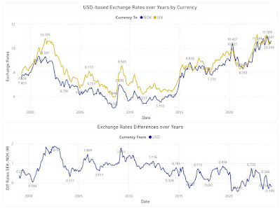
Certain operations require comparing the trends of two currencies. The first plot shows the evolution NOK and SEK in respect to EUR, while the second shows only the differences between the two XRs:

The first plot will show different values when performed against other currency (e.g. USD), however the second plot will look similarly, even if the points deviate slightly:

Another important difference is the one between monthly and yearly XRs, difference depicted by the below plot:

The value differences between the two XR types can have considerable impact on reporting. Therefore, one must reflect in analyses the rate type used in the actual process. 

Attempting to project data into the future can require complex techniques, however, sometimes is enough to highlight a probable area, which depends also on the confidence interval (e.g. 85%) and the forecast length (e.g. 10 months):

Every perspective into the data tends to provide something new that helps in sense-making. For some users the first table with flexible filtering (e.g. time unit, currency type, currency from/to) is enough, while for others multiple perspectives are needed. When possible, one should  allow users to explore the various perspectives and use the feedback to remove or even add more perspectives. Including a feedback loop in graphical representation is important not only for tailoring the visuals to users' needs but also for managing their expectations,  respectively of learning what works and what doesn't.

Comments:
1) I used GBP to NOK XRs to provide an example based on  triangulation.
2) Some experts advise against using borders or grid lines. Borders, as the name indicates allow to delimitate between various areas, while grid lines allow to make comparisons within a section without needing to sway between broader areas, adding thus precision to our senses-making. Choosing grey as color for the elements from the background minimizes the overhead for coping with more information while allowing to better use the available space.
3) Trend lines are recommended where the number of points is relatively small and only one series is involved, though, as always, there are exceptions too. 
4) In heatmaps one can use a gradient between two colors to show the tendencies of moving toward an extreme or another. One should avoid colors like red or green.
5) Ideally, a color should be used for only one encoding (e.g. one color for the same month across all graphics), though the more elements need to be encoded, the more difficult it becomes to respect this rule. The above graphics might slightly deviate from this as the purpose is to show a representation technique. 
6) In some graphics the XRs are displayed only with two decimals because currently the technique used (visual calculations) doesn't support formatting.
7) All the above graphical elements are based on a Power BI solution. Unfortunately, the tool has its representational limitations, especially when one wants to add additional information into the plots. 
8) Unfortunately, the daily XR values are not easily available from the same source. There are special scenarios for which a daily, hourly or even minute-based analysis is needed.
9) It's a good idea to validate the results against the similar results available on the web (see the ECB website).

Previous Post <<||>> Next Post

🪄SSRS: Graphical Representations II (Sixth Magic Class)

Introduction 

Using a single chart to display multiple series in SQL Server Reporting Services (SSRS) or any other reporting tool works well when the number of series is somehow manageable - usually being enough to display 2-10 series within the same chart. The more series one adds, the more complicated will be for users to read the chart. One has the choice to find either
-  a level of detail (e.g. Category) which, when grouping the data, leads to a number of manageable series,

-  compare the data within a certain grouping (e.g. Category),

-  displaying the individual trends (e.g. for each Product). 

Let's consider the last choice. The report from this post will display the Sales Volume per Product and Year/Month of the Sales Orders available in the AdventureWorks2014 database. The logic uses the Sales.SalesOrderDetail and Sales.SalesOrderHeader tables, respectively the Production.vProducts view created in a previous post. 

Note:

A Sales Volume report is more appropriate to be built using a data warehouse's data, which are already aggregated and prepared for such reports. There's actually an AdventureWorksDW2014 data warehouse model made available which can be used to display the same information, however the intent is to demonstrate the techniques of working with data in an OLTP environment. 

Preparing the Data

Creating a view to build the Sales Orders details is usually recommended, though for the current report we just need the Product Category, Subcategory, Number and Name, respectively Sales Date, Quantity and Value, which is only a small part from the attributes available. Another choice to consider is whether to use the raw data, though then the number of records sent to the client can be considerably high, or aggregate the data and the lowermost level of detail needed for the report, in this case the Category, Subcategory, Product, Month and Year:

-- Sales volume per Product   
SELECT ITM.Category
, ITM.Subcategory
, ITM.ProductNumber
, ITM.Name
, Month(SOH.OrderDate) [Month]
, Year(SOH.OrderDate) [Year]
, Sum(SOD.OrderQty) OrderQty
, Sum(SOD.LineTotal) OrderValue
FROM Sales.SalesOrderDetail SOD
     JOIN Sales.SalesOrderHeader SOH
       ON SOD.SalesOrderID = SOH.SalesOrderID
     JOIN Production.vProducts ITM
       ON SOD.ProductId = ITM.Productid 
WHERE ITM.ProductNumber IN ('BB-7421', 'BB-9108')
GROUP BY ITM.Category
, ITM.Subcategory
, ITM.ProductNumber
, ITM.Name
, Month(SOH.OrderDate)
, Year(SOH.OrderDate)
ORDER BY ITM.Category
, ITM.Subcategory
, ITM.ProductNumber
, [Year]
, [Month]

The query contains all the needed data, however one could have more flexibility if the data would contain cumulative or total values as well: 

-- Sales volume per Product (extended)  
SELECT SOD.Category
, SOD.Subcategory
, SOD.ProductNumber
, SOD.Name
, SOD.[Month]
, SOD.[Year]
, SOD.OrderQty
, SOD.OrderValue
, SUM(SOD.OrderQty) OVER (PARTITION BY SOD.ProductNumber) TotalQty
, SUM(SOD.OrderValue) OVER (PARTITION BY SOD.ProductNumber) TotalValue
, SUM(SOD.OrderQty) OVER (PARTITION BY SOD.ProductNumber ORDER BY [Year], [Month]) CumulatedQty
, SUM(SOD.OrderValue) OVER (PARTITION BY SOD.ProductNumber ORDER BY [Year], [Month]) CumulatedValue
FROM (-- cumulated values
 SELECT ITM.Category
 , ITM.Subcategory
 , ITM.ProductNumber
 , ITM.Name
 , Month(SOH.OrderDate) [Month]
 , Year(SOH.OrderDate) [Year]
 , Sum(SOD.OrderQty) OrderQty
 , Sum(SOD.LineTotal) OrderValue
 FROM Sales.SalesOrderDetail SOD
   JOIN Sales.SalesOrderHeader SOH
    ON SOD.SalesOrderID = SOH.SalesOrderID
   JOIN [Production].[vProducts] ITM
     ON SOD.ProductId = ITM.Productid 
 WHERE ITM.ProductNumber IN ('BB-7421', 'BB-9108')
 GROUP BY ITM.Category
    , ITM.Subcategory
 , ITM.ProductNumber
 , ITM.Name
 , Month(SOH.OrderDate)
 , Year(SOH.OrderDate)
  ) SOD
ORDER BY SOD.Category
, SOD.Subcategory
, SOD.ProductNumber
, SOD.[Year]
, SOD.[Month]

In the end one can use any of the above queries.
Note:When prototyping a report is usually recommended to consider only a small number of records (e.g. only two Products). In addition, do not forget to validate the number or records considered by the logic:

-- checking the view for internal data consistency
SELECT count(*)
FROM Sales.SalesOrderDetail SOD
     JOIN Sales.SalesOrderHeader SOH
   ON SOD.SalesOrderID = SOH.SalesOrderID
  JOIN Production.vProducts ITM
    ON SOD.ProductId = ITM.Productid 

Creating the Report
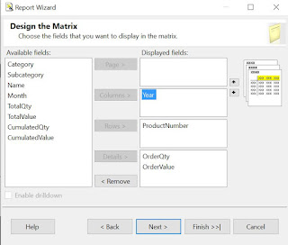
Using the Report Wizard create a new matrix report called "Sales Volume per Product" based on either of the above queries (I considered the second). Within "Design the Matrix" select the attributes as follows:

Design the Matrix

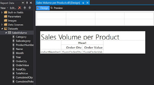
This will create the backbone for our report:

First draft in Design mode

Which is pretty basic, if we consider the output:

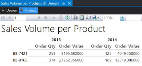
First draft in Preview mode

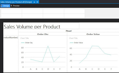
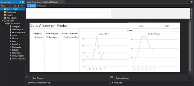
Now, returning in Design mode, right click on the "Sum of OrderQty" cell and from the floating menu select Insert/Chart, while from the list of available charts select Line. Do the same for "Sum of OrderValue". And here's the result:

Second draft in Design mode

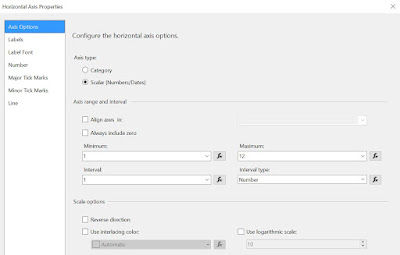
As only one series will be displayed, select the Chart Title and delete the respective label. Delete the Series label as well. When running the report you'll observe that the horizontal axis values are not really appealing. To dix this right click on the respective area and from the floating menu select Horizontal Axis Properties. Within Axis Options section change the Axis type as 'Scalar', enter '1' as Minimum, '12' as Maximum, '1' as Interval and 'Number' as Interval type:

Horizontal Axis Properties

In the same window, within the Labels section select 'Enable auto-fit' and uncheck the "Labels can be offset", respectively the "Labels can be rotated" checkboxes. 

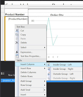
To include the Category, Subcategory and eventually the Product Name, select the Product Number cell, right click on it, and from the floating menu select Insert Column/Inside Group - Left, then select from the Category as attribute:

Inserting a column within the group

Repeat the process to add the Subcategory. Eventually you can add also the Product Name, though for it you'll have to select "Inside Group - Right". 

To improve the design, you can add a Page Header and move the report's title into it add a timestamp, respectively a page count textbox, resize the boxes to fit the columns. You can also align the column header values to the center, change the font to 10pt, etc.

Third draft in Design mode

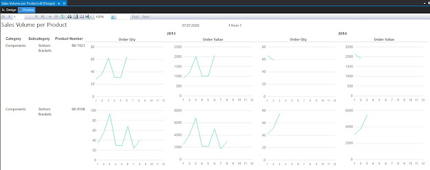
Here's the report in preview mode:

Third draft in Preview mode

One can use the report the way it is, or add the Category and Subcategory as parameters. Similarly, one can use the cumulative values as input for the charts. 

Revamping the Report with Sparklines

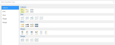
Even if the charts allow displaying the scales, the problem with them is that they are too big, which makes it difficult to compare the data across records. One can correct this by using the other types of graphics available in reports, e.g. sparklines. For this make a copy of the report already built, and within the Detail cells select a Sparkine Column instead of a chart:

Sparkline types

In comparison with Lines, Column-based representations allow to see how many data points are represented. Because spartklines are more compact as graphic forms, you can resize the cells as follows:

Fourth draft in Design mode

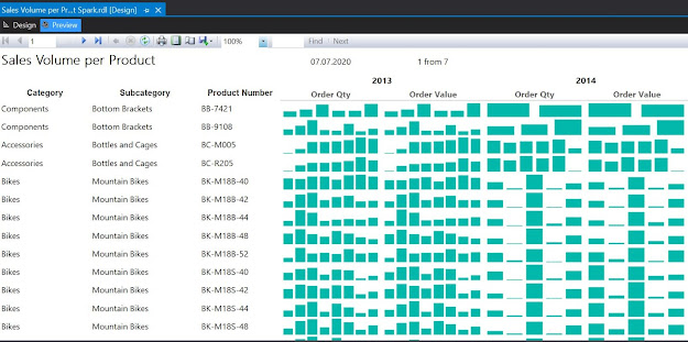
And here's the report in preview mode (the constraints from the source query were removed):

Fourth draft in Preview mode

As can be seen one can easily identify the trends however the volume scale was lost, being impossible to compare which of the Products sold better. One can bring the Total Quantity and Value as display information and sort the dataset from the highest to lowest value. One can even select a top x, to reduce the focus only to the most sold Products.

If the prices remained relatively constant over time, there's actually almost no difference between the graphic displays for Order Quantity, respectively for Order Value. Therefore one can remove one of them (e.g. Order Quantity). Being more compact, sparkline-based representations allow to better use the space, therefore you can add more fields into the report. 

Happy coding!

📉Graphical Representation: Sparklines (Just the Quotes)

"A sparkline is a small, intense, simple, word-sized graphic with typographic resolution. Sparklines mean that graphics are no longer cartoonish special occasions with captions and boxes, but rather sparkline graphics can be everywhere a word or number can be: embedded in a sentence, table, headline, map, spreadsheet, graphic." (Edward R Tufte, "Beautiful Evidence", 2006)

"By segregating evidence by mode (word, number, image, graph), the current-day computer approach contradicts the spirit of sparklines, a spirit that makes no distinction among words, numbers, graphics, images. It is all evidence, after all. A good system for evidence display should be centered on evidence, not on a collection of application programs each devoted to a single mode of information." (Edward R Tufte, "Beautiful Evidence", 2006)

"By showing recent change in relation to many past changes, sparklines provide a context for nuanced analysis - and, one hopes, better decisions. [...] Sparklines efficiently display and narrate binary data (presence/absence, occurrence/non-occurrence, win/loss). [...] Sparklines can simultaneously accommodate several variables. [...] Sparklines can narrate on-going results detail for any process producing sequential binary outcomes." (Edward R Tufte, "Beautiful Evidence", 2006)

"Sparklines are word-like graphics, With an intensity of visual distinctions comparable to words and letters. [...] Words visually present both an overall shape and letter-by-letter detail; since most readers have seen the word previously, the visual task is usually one of quick recognition. Sparklines present an overall shape and aggregate pattern along with plenty of local detail. Sparklines are read the same way as words, although much more carefully and slowly." (Edward R Tufte, "Beautiful Evidence", 2006)

"Sparklines vastly increase the amount of data within our eye-span and intensify statistical graphics up to the everyday routine capabilities of the human eye-brain system for reasoning about visual evidence, seeing distinctions, and making comparisons. [...] Providing a straightforward and contextual look at intense evidence, sparkline graphics give us some chance to be approximately right rather than exactly wrong."  (Edward R Tufte, "Beautiful Evidence", 2006)

"Sparklines work at intense resolutions, at the level of good typography and cartography. [...] Just as sparklines are like words, so then distributions of sparklines on a page are like sentences and paragraphs. The graphical idea here is make it word-like and typographic - an idea that leads to reasonable answers for most questions about sparkline arrangements." (Edward R Tufte, "Beautiful Evidence", 2006)

"These little data lines, because of their active quality over time, are named sparklines - small, high-resolution graphics usually embedded in a full context of words, numbers, images. Sparklines are data words: data-intense, design-simple, word-sized graphics." (Edward R Tufte, "Beautiful Evidence", 2006)

"Sparklines are compact line graphs that do not have a quantitative scale. They are meant to provide a quick sense of a metric's movement or trend, usually over time. They are more expressive than arrows, which only indicate change from the prior period and do not qualify the degree of change. Sparklines are significantly more compact than normal line graphs but are precise." (Wayne W Eckerson, "Performance Dashboards: Measuring, Monitoring, and Managing Your Business", 2010)

"The biggest difference between line graphs and sparklines is that a sparkline is compact with no grid lines. It isn't meant to give precise values; rather, it should be considered just like any other word in the sentence. Its general shape acts as another term and lends additional meaning in its context. The driving forces behind these compact sparklines are speed and convenience." (Brian Suda, "A Practical Guide to Designing with Data", 2010)

"Sparklines aren't necessarily a variation on the line chart, rather, a clever use of them. [...] They take advantage of our visual perception capabilities to discriminate changes even at such a low resolution in terms of size. They facilitate opportunities to construct particularly dense visual displays of data in small space and so are particularly applicable for use on dashboards." (Andy Kirk, "Data Visualization: A successful design process", 2012)

"Line graphs that show more than one line can be useful for making comparisons, but sometimes it is important to discuss each individual line. By using sparklines evaluators can call attention to and discuss individual cases. Sparklines can be embedded within a sentence to illustrate a trend and help stakeholders better understand the data. Evaluators can use this simple visualization when creating reports." (Christopher Lysy, "Developments in Quantitative Data Display and Their Implications for Evaluation", 2013)

"Using sparklines is not as simple as it might seem. You must ensure that variation is as clear as possible. […] Sparklines are an interesting concept, but there are a few issues associated with their extreme miniaturization, among which is the removal of the vertical axes and the consequent absence of quantitative references." (Jorge Camões, "Data at Work: Best practices for creating effective charts and information graphics in Microsoft Excel", 2016)

"Sparklines focus on the trend over time and the direction rather than the actual values. Sparklines are used to visualize volatility or outliers. They are usually kept quite narrow on dashboards but still maintain an aspect ratio of 2:3." (Lorna Brown, "Tableau Desktop Cookbook", 2020)

📈Graphical Representation: Sparklines (Definitions)

"A sparkline is a small, intense, simple, word-sized graphic with typographic resolution." (Edward R Tufte, "Beautiful Evidence", 2006)

"A sparkline is a mini-image (thumbnail) of graphical data that enables you to put numbers in a temporal context without the need to display full charts." (Brian Clifton, "Advanced Web Metrics with Google Analytics", 2010)

"A sparkline is a very small chart, typically a line chart, that is drawn without labels on either axis. Its purpose is to show the variation in data, typically over time." (Bruce Johnson, "Professional Visual Studio", 2012)

"Sparklines are condensed graphs or charts that can be used in-line with text or grouped to show trends across several different measures." (Ryan Sleeper, "Practical Tableau: 100 Tips, Tutorials, and Strategies from a Tableau Zen Master", 2018)

"A sparkline is a small line chart with the purpose of showing a general trend, without the full details. A sparkline is very efficient in the amount of screen space it uses." (Andrew Berridge &, Michael Phillips, "TIBCO Spotfire: A Comprehensive Primer", 2019)

"A Sparkline is a tiny chart that appears in a cell and does not include any text data. So, a Sparkline is a great way to give a quick glance of a trend." (Eric Butow, "MCA Microsoft Office Specialist: Office 365 and Office 2019", 2021)

"A sparkline chart is a small, simple, and condensed data visualization tool that presents trends and variations in data over a concise space, typically in the form of a tiny line chart." (Phocas)

"A sparkline is a line chart that displays the variation in a null value, unique value, or non-unique value across the latest five consecutive profile runs." (Informatica)

"A sparkline is a tiny chart in a worksheet cell that provides a visual representation of data. Use sparklines to show trends in a series of values, such as seasonal increases or decreases, economic cycles, or to highlight maximum and minimum values. Position a sparkline near its data for greatest impact." (Microsoft)

"A sparkline is a very small line chart, typically drawn without axes or coordinates. It presents the general shape of a variation (typically over time) in some measurement, such as temperature or stock market price, in a simple and highly condensed way." (Wikipedia)

"Sparklines are small, simple line graphs traditionally used for displaying trends or variations of some variable" (TIBCO)