⚡️Power BI: Working with Visual Calculations (Part III: Matrix Tables with Square Numbers as Example)

Introduction

In the previous post I exemplified various operations that can be performed with visual calculations on simple tables based on square numbers. Changing the simple table to a matrix table doesn't bring any benefit. The real benefit comes when one restructures the table to store only a cell per row in a table. 

Data Modelling

For this the Magic5 table can be transformed via the following code, which creates a second table (e.g. M5):

M5 = UNION (
    SUMMARIZECOLUMNS(
     Magic5[Id]
     , Magic5[R]
     , Magic5[Index]
     , Magic5[C1]
     , "Col", "C1"
    )
    , SUMMARIZECOLUMNS(
     Magic5[Id]
     , Magic5[R]
     , Magic5[Index]
     , Magic5[C2]
     , "Col", "C2"
    )
    , SUMMARIZECOLUMNS(
     Magic5[Id]
     , Magic5[R]
     , Magic5[Index]
     , Magic5[C3]
     , "Col", "C3"
    )
    ,  SUMMARIZECOLUMNS(
     Magic5[Id]
     , Magic5[R]
     , Magic5[Index]
     , Magic5[C4]
     , "Col", "C4"
    )
    , SUMMARIZECOLUMNS(
      Magic5[Id]
     , Magic5[R]
     , Magic5[Index]
     , Magic5[C5]
     , "Col", "C5"
    )
)

Once this done, one can add the column [Col] as values for the matrix in a new visual. From now on, all the calculations can be done on copies of this visual. 

Simple Operations

The behavior of the RUNNINGSUM and other functions is different when applied on a matrix table because the formula is applied to every cell of the N*N table, a column with the result being added for each existing column of the matrix.

Moreover, there are four different ways of applying the formula based on the Axis used. ROW calculates the formula by the row within a column:

Run SumByRow(C) = RUNNINGSUM([C], ROWS)

Output:

R	C	Run Sum(C)	C	Run Sum(C)	C	Run Sum(C)	C	Run Sum(C)	C	Run Sum(C)
R1	18	18	25	25	2	2	9	9	11	11
R2	4	22	6	31	13	15	20	29	22	33
R3	15	37	17	48	24	39	1	30	8	41
R4	21	58	3	51	10	49	12	42	19	60
R5	7	65	14	65	16	65	23	65	5	65

By providing COLUMNS as parameter for the Axis makes the calculation run by the column within a row: 

Run SumByCol(C) = RUNNINGSUM([C], COLUMNS)

Output:

R	C	Run Sum(C)	C	Run Sum(C)	C	Run Sum(C)	C	Run Sum(C)	C	Run Sum(C)
R1	18	18	25	43	2	45	9	54	11	65
R2	4	4	6	10	13	23	20	43	22	65
R3	15	15	17	32	24	56	1	57	8	65
R4	21	21	3	24	10	34	12	46	19	65
R5	7	7	14	21	16	37	23	60	5	65

By providing ROW COLUMNS as parameter for the Axis makes the calculation run by the column and then continuing the next column (without resetting the value at the end of the column):

Run SumByRow-Col(C) = RUNNINGSUM([C],ROWS COLUMNS)

Output:

R	C	Run Sum(C)	C	Run Sum(C)	C	Run Sum(C)	C	Run Sum(C)	C	Run Sum(C)
R1	18	18	25	90	2	132	9	204	11	271
R2	4	22	6	96	13	145	20	224	22	293
R3	15	37	17	113	24	169	1	225	8	301
R4	21	58	3	116	10	179	12	237	19	320
R5	7	65	14	130	16	195	23	260	5	325

By providing COLUMNS ROWS as parameter for the Axis makes the calculation run by the row and then continuing the next row (without resetting the value at the end of the column):

Run SumByCol-Row = RUNNINGSUM([C],COLUMNS ROWS)

Output:

R	C	Run Sum(C)	C	Run Sum(C)	C	Run Sum(C)	C	Run Sum(C)	C	Run Sum(C)
R1	18	18	25	43	2	45	9	54	11	65
R2	4	69	6	75	13	88	20	108	22	130
R3	15	145	17	162	24	186	1	187	8	195
R4	21	216	3	219	10	229	12	241	19	260
R5	7	267	14	281	16	297	23	320	5	325

Ranking

RANK can be applied independent of the values, or considering the value with ASC or DESC sorting:

RankByRow = RANK(DENSE,ROWS) -- ranking by row independent of values
RankByRow ASC = RANK(DENSE,ROWS, ORDERBY([C],ASC)) -- ranking by row ascending
RankByRow DESC = RANK(DENSE,ROWS, ORDERBY([C], DESC)) -- ranking by row descending
RankByRow-Col ASC = RANK(DENSE,ROWS COLUMNS, ORDERBY([C],ASC)) -- ranking by row columns ascending
RankByRow-Col DESC = RANK(DENSE,ROWS COLUMNS, ORDERBY([C], DESC)) -- ranking by row columns ascending

[RankByRow-Col ASC] matches the actual numbers from the matrix and is thus useful when sorting any numbers accordingly. 

Differences

Differences can be calculated between any of the cells of the matrix:

DiffToPrevByRow = [C] - PREVIOUS([C])  -- difference to previous record
DiffToPrevByRow* = IF(NOT(IsBlank(PREVIOUS([C]))), [C] - PREVIOUS([C])) -- extended difference to previous record
DiffToPrevByRow-Col = [C] - PREVIOUS([C],, ROWS COLUMNS) -- difference to previous record by ROWS COLUMNS
DiffToFirstByRow = [C] - FIRST([C]) -- difference to first record
DiffToPrevByCol = [C] - FIRST([C], COLUMNS) -- difference to previous record COLUMNS

Ranking = RANK(DENSE, ROWS COLUMNS, ORDERBY([C], ASC)) -- ranking of values by ROWS COLUMNS
OffsetDiffToPrevByRow = [C] - calculate([C], OFFSET(1, ROWS, ORDERBY([Ranking],DESC))) -- difference to the previous record by ROW
OffsetDiffToPrevByRow-Col = [C] - calculate([C], OFFSET(1, ROWS COLUMNS, ORDERBY([Ranking],DESC))) -- difference to the previous record by ROW

Ranking has been introduced to facilitate the calculations based on OFFSET.

The other functions [1] can be applied similarly.

Happy coding!

Previous Post <<||>> Next Post

References:
[1] Microsoft Learn (2024) Power BI: Using visual calculations [preview] (link)

⚡️Power BI: Working with Visual Calculations (Part II: Simple Tables with Square Numbers as Example)

Introduction

The records behind a visual can be mentally represented as a matrix, the visual calculations allowing to tap into this structure intuitively and simplify many of the visualizations used. After a general test drive of the functionality, it makes sense to dive deeper into the topic to understand more about the limitations, functions behavior and what it takes to fill the gaps. This post focuses on simple tables, following in a next post to focus on matrices and a few other topics. 

For exemplification, it makes sense to use a simple set of small numbers that are easy to work with, and magic squares seem to match this profile. A magic square is a matrix of positive sequential numbers in which each row, each column, and both main diagonals are the same [1]. Thus, a square of order N has N*N numbers from 1 to N*N, the non-trivial case being order 3. However, from the case of non-trivial squares, the one of order 5 provides a low order and allows hopefully the minimum needed for exemplification:

18	25	2	9	11
4	6	13	20	22
15	17	24	1	8
21	3	10	12	19
7	14	16	23	5
1	7	13	19	25

Data Modeling

One magic square should be enough to exemplify the various operations, though for testing purposes it makes sense to have a few more squares readily available. Each square has an [Id], [C1] to [C5] corresponds to matrix's columns, while [R] stores a row identifier which allows to sort the values the way they are stored in the matrix:

let
    Source = #table({"Id","C1","C2","C3","C4","C5","R"}
, {
{1,18,25,2,9,11,"R1"},
{1,4,6,13,20,22,"R2"},
{1,15,17,24,1,8,"R3"},
{1,21,3,10,12,19,"R4"},
{1,7,14,16,23,5,"R5"},
{2,1,7,13,19,25,"R1"},
{2,14,20,21,2,5,"R2"},
{2,22,3,9,15,16,"R3"},
{2,10,11,17,23,4,"R4"},
{2,18,24,5,6,12,"R5"},
{3,1,2,22,25,15,"R1"},
{3,9,10,16,11,19,"R2"},
{3,17,23,13,5,7,"R3"},
{3,24,12,6,20,3,"R4"},
{3,14,18,8,4,21,"R5"},
{4,22,6,3,18,16,"R1"},
{4,4,14,11,15,21,"R2"},
{4,5,8,12,23,17,"R3"},
{4,25,13,19,7,1,"R4"},
{4,9,24,20,2,10,"R5"},
{5,5,9,20,25,6,"R1"},
{5,13,15,2,11,24,"R2"},
{5,21,1,23,3,17,"R3"},
{5,19,18,4,14,10,"R4"},
{5,7,22,16,12,8,"R5"}
}
),
    #"Changed Type to Number" = Table.TransformColumnTypes(Source,{{"C1", Int64.Type}, {"C2", Int64.Type}, {"C3", Int64.Type}, {"C4", Int64.Type}, {"C5", Int64.Type}}),
    #"Sorted Rows" = Table.Sort(#"Changed Type to Number",{{"Id", Order.Ascending}, {"R", Order.Ascending}}),
    #"Added Index" = Table.AddIndexColumn(#"Sorted Rows", "Index", 0, 1, Int64.Type)
in
    #"Added Index"

The column names and the row identifier could have been numeric values from 1 to 5, though it could have been confounded with the actual numeric values.

In addition, the columns [C1] to [C5] were formatted as integers and an index was added after sorting the values after [Id] and [R]. Copy the above code as a Blank Query in Power BI and change the name to Magic5. 

Prerequisites

For the further steps you'll need to enable visual calculations in Power BI Developer via:
File >> Options and settings >> Options >> Preview features >> Visual calculations >> (check)

Into a Table visual drag and drop [R], [C1] to [C5] as column and make sure that the records are sorted ascending by [R]. To select only a square, add a filter based on the [Id] and select the first square. Use further copies of this visual for further tests. 

Some basic notions of Algebra are recommended but not a must. If you worked with formulas in Excel, then you are set to go. 

In Mathematics a matrix starts from the top left side and one moves on the rows (e.g. 18, 25, 2, ...) and then on the columns. With a few exceptions in which the reference is based on the latest value from a series (see Exchange rates), this is the direction that will be followed. 

Basic Operations

Same as in Excel [C1] + [C2] creates a third column in the matrix that stores the sum of the two. The sum can be further applies to all the columns:

Sum(C) = [C1] + [C2] + [C3] + [C4] + [C5] -- sum of all columns (should amount to 65)

The column can be called "Sum", "Sum(C)" or any other allowed unique name, though the names should be meaningful, useful, and succinct, when possible.

Similarly, one can work with constants, linear or nonlinear transformations (each formula is a distinct calculation):

constant = 1 -- constant value
linear = 2*[C1] + 1 -- linear translation: 2*x+1

linear2 = 2*[C1] + [constant] -- linear translation: 2*x+1
quadratic = Power([C1],2) + 2*[C1] + 1 -- quadratic translation: x^2+2*x+1
quadratic2 = Power([C1],2) + [linear] -- quadratic translation: x^2+2*x+1

Output:

R	C1	constant	linear	linear2	quadratic	quadratic2
R1	18	1	37	37	361	361
R2	4	1	9	9	25	25
R3	15	1	31	31	256	256
R4	21	1	43	43	484	484
R5	7	1	15	15	64	64

Please note that the output was duplicated in Excel (instead of making screenshots).

Similarly, can be build any type of formulas based on one or more columns.

With a simple trick, one can use DAX functions like SUMX, PRODUCTX, MINX or MAXX as well:

Sum2(C) = SUMX({[C1], [C2], [C3], [C4], [C5]}, [Value]) -- sum of all columns

Prod(C) = PRODUCTX({[C1], [C2], [C3], [C4], [C5]}, [Value]) -- product of all columns

Avg(C) = AVERAGEX({[C1], [C2], [C3], [C4], [C5]}, [Value]) -- average of all columns

Min(C) = MINX({[C1], [C2], [C3], [C4], [C5]}, [Value]) -- minimum value of all columns

Max(C) = MAXX({[C1], [C2], [C3], [C4], [C5]}, [Value]) -- maximum value of all columns
Count(C) = COUNTX({[C1], [C2], [C3], [C4], [C5]},[Value]) -- counts the number of columns

Output:

C1	C2	C3	C4	C5	Sum(C)	Avg(C)	Prod(C)	Min(C)	Max(C)	Count(C)
18	25	2	9	11	65	13	89100	2	25	5
4	6	13	20	22	65	13	137280	4	22	5
15	17	24	1	8	65	13	48960	1	24	5
21	3	10	12	19	65	13	143640	3	21	5
7	14	16	23	5	65	13	180320	5	23	5

Unfortunately, currently there seems to be no way available for applying such calculations without referencing the individual columns. 

Working across Rows

ROWNUMBER and RANK allow to rank a cell within a column independently, respectively dependently of its value:

Ranking = ROWNUMBER() -- returns the rank in the column (independently of the value)
RankA(C) = RANK(DENSE, ORDERBY([C1], ASC)) -- ranking of the value (ascending) 

RankD(C) = RANK(DENSE, ORDERBY([C1], DESC)) -- ranking of the value (descending) 

Output:

R	C1	Ranking	RankA(C)	RankD(C)
R1	18	1	4	2
R2	4	2	1	5
R3	15	3	3	3
R4	21	4	5	1
R5	7	5	2	4

PREVIOUS, NEXT, LAST and FIRST allow to refer to the values of other cells within the same column:

Prev(C) = PREVIOUS([C1]) -- previous cell
Next(C) = NEXT([C1])  -- next cell

First(C) = FIRST([C1]) -- first cell
Last(C) = LAST([C1]) -- last cell

Output:

R	C1	Prev(C)	NextC)	First(C)	Last(C)
R1	18		4	18	7
R2	4	18	15	18	7
R3	15	4	21	18	7
R4	21	15	7	18	7
R5	7	21		18	7

OFFSET is a generalization of these functions

offset(2) = calculate([C1], offset(2)) -- 
offset(-2) = calculate([C1], offset(-2))
Ind = ROWNUMBER() -- index
inverse = calculate([C1], offset(6-2*[Ind])) -- inversing the values based on index

Output:

R	C1	offset(2)	offset(-2)	ind	inverse
R1	18	15		1	7
R2	4	21		2	21
R3	15	7	18	3	15
R4	21		4	4	4
R5	7		15	5	18

The same functions allow to calculate the differences for consecutive values:

DiffToPrev(C) = [C1] - PREVIOUS([C1]) -- difference to previous 
DiffToNext(C) = [C1] - PREVIOUS([C1]) -- difference to next 
DiffTtoFirst(C) = [C1] - FIRST([C1]) -- difference to first
DiffToLast(C) = [C1] - LAST([C1]) -- difference to last

Output:

R	C1	DiffToPrev(C)	DiffToNextC)	DiffToFirst(C)	DiffToLast(C)
R1	18	18	14	0	11
R2	4	-14	-11	-14	-3
R3	15	11	-6	-3	8
R4	21	6	14	3	14
R5	7	-14	7	-11	0

DAX makes available several functions for working across the rows of the same column. Two of the useful functions are RUNNINGSUM and MOVINGAVERAGE:

Run Sum(C) = RUNNINGSUM([C1]) -- running sum

Moving Avg3(C) = MOVINGAVERAGE([C1], 3) -- moving average for the past 3 values

Moving Avg2(C) = MOVINGAVERAGE([C1], 2) -- moving average for the past 2 values

Unfortunately, one can use only the default sorting of the table with the functions that don't support the ORDERBY parameter. Therefore, when the table needs to be sorted descending and the RUNNINGSUM calculated ascending, for the moment there's no solution to achieve this behavior. However, it appears that Microsoft is planning to implement a solution for this issue.

RUNNINGSUM together with ROWNUMBER can be used to calculate a running average:

Run Avg(C) = DIVIDE(RUNNINGSUM([C1]), ROWNUMBER()) -- running average

Output:

R	C1	Run Sum(C)	Moving Avg3(C)	Moving Avg2(C)	Run Avg(C)
R1	18	18	18	18	18
R2	4	22	11	11	11
R3	15	37	12.33	9.5	12.33
R4	21	58	13.33	18	14.5
R5	7	65	14.33	14	13

With a mathematical trick that allows to transform a product into a sum of elements by applying the Exp (exponential) and Log (logarithm) functions (see the solution in SQL), one can run the PRODUCT across rows, though the values must be small enough to allow their multiplication without running into issues:

Ln(C) = IFERROR(LN([C1]), Blank()) -- applying the natural logarithm
Sum(Ln(C)) = RUNNINGSUM([Ln(C)]) -- running sum
Run Prod(C) = IF(NOT(ISBLANK([Sum(Ln(C))])), Exp([Sum(Ln(C))])) -- product across rows

Output:

R	C1	Ln(C)	Sum(Ln(C))	Run Prod(C)
R1	18	2.89	2.89	18
R2	4	1.39	4.28	72
R3	15	2.71	6.98	1080
R4	21	3.04	10.03	22680
R5	7	1.95	11.98	158760

These three calculations could be brought into a single formula, though the result could be more difficult to troubleshoot. The test via IsBlank is necessary because otherwise the exponential for the total raises an error. 

Considering that when traversing a column it's enough to remember the previous value, one can build MIN and MAX functionality across a column: 

Run Min = IF(OR(Previous([C1]) > [C1], IsBlank(Previous([C1]))), [C1], Previous([C1])) -- minimum value across rows
Run Max = IF(OR(Previous([C1]) < [C1], IsBlank(Previous([C1]))), [C1], Previous([C1])) -- maximum across rows

Happy coding!

Previous Post <<||>> Next Post

References:
[1] Wikipedia (2024) Magic Squares (online)
[2] Microsoft Learn (2024) Power BI: Using visual calculations [preview] (link)

⚡️🗒️Power BI: Working with Visual Calculations (Part I: Test Drive) [new feature]

Introduction

I recently watched a webcast with Jeroen (Jay) ter Heerdt (see [2]) in which he introduces visual calculations, a type of DAX calculation that's defined and executed directly on a visual [1]. Visual calculations provide an approach of treating a set of data much like an Excel table, allowing to refer to any field available on a visual and write formulas, which simplifies considerably the solutions used currently for ranking records, running averages and other windowing functions. 

The records behind a visual can be mentally represented as a matrix, while the visual calculations can refer to any column from the matrix, allowing to add new columns and include the respective columns in further calculations. Moreover, if a column is used in a formula, it's not recalculated as is the case of measures, which should improve the performance of DAX formulas considerably. 

Currently, one can copy a formula between visuals and if the formula contains fields not available in the targeted visual, they are added as well. Conversely, it's possible to build such a visual, copy it and then replace the dimension on which the analysis is made (e.g. Customer with Product), without being needed to make further changes. Unfortunately, there are also downsides: (1) the calculations are visible only within the visual in which were defined; (2) currently, the visual's data can't be exported if a visual calculation is added; (3) no formatting is supported, etc.

Ranking and Differences

I started to build a solution based on publicly available sales data, which offers a good basis for testing the use of visual calculations. Based on a Power BI visual table made of [Customer Name], [Sales Amount], [Revenue] and [Total Discount], I've added several calculations:

-- percentages
Sales % = 100*DIVIDE([Sales Amount], COLLAPSE([Sales Amount], ROWS))
Revenue % = 100*DIVIDE([Revenue],[Sales Amount])
Discount % = 100*DIVIDE([Total  Discount], [Total  Discount]+[Sales Amount])

-- rankings 
Rank Sales = Rank(DENSE, ORDERBY([Sales Amount], DESC))
Rank Revenue = Rank(DENSE, ORDERBY([Revenue], DESC))

-- differences between consecutive values
Diff. to Prev. Sales = IF([Rank Sales]>1, INDEX([Rank Sales]-1, , ORDERBY([Sales Amount], DESC)) - [Sales Amount] , BLANK())
Diff. to Prev. Rev. = IF([Rank Revenue]>1, INDEX([Rank Revenue]-1, , ORDERBY([Revenue], DESC)) - [Revenue] , BLANK())

Here's the output considered only for the first 10 records sorted by [Sales Amount]:

Customer Name	Sales Amount	Sales %	Revenue	Revenue %	Total Discount	Discount %	Rank Sales	Diff. to Prev. Sales.	Rank Rev.	Diff. to Prev. Rev.
Medline	1058923.78	3.76	307761.99	3.75	126601.02	10.68	1		1
Ei	707663.21	2.51	229866.98	2.8	95124.09	11.85	2	351260.57	2	77895.01
Elorac, Corp	702911.91	2.49	209078.76	2.55	83192.39	10.58	3	4751.3	6	20788.22
Sundial	694918.98	2.47	213362.1	2.6	78401.72	10.14	4	7992.93	4	-4283.34
OUR Ltd	691687.4	2.45	196396.26	2.4	78732.2	10.22	5	3231.58	10	16965.84
Eminence Corp	681612.78	2.42	213002.78	2.6	86904.03	11.31	6	10074.62	5	-16606.52
Apotheca, Ltd	667283.99	2.37	157435.56	1.92	101453.91	13.2	7	14328.79	31	55567.22
Rochester Ltd	662943.9	2.35	224918.2	2.74	81158.11	10.91	8	4340.09	3	-67482.64
ETUDE Ltd	658370.48	2.34	205432.79	2.51	89322.72	11.95	9	4573.42	9	19485.41
Llorens Ltd	646779.31	2.29	206567.4	2.52	82897.59	11.36	10	11591.17	8	-1134.61

Comments:
1) One could use [Total Amount] = [Total  Discount]+[Sales Amount] as a separate column.
2) The [Rank Sales] is different from the [Rank Rev.] because of the discount applied.
3) In the last two formulas a blank was considered for the first item from the ranking.
4) It's not possible to control when the totals should be displayed, however one can change the color for the not needed total to match the background.

Visualizing Differences 

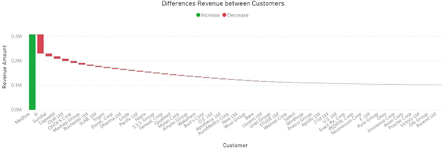
Once the formulas are added, one can hide the basis columns and visualize the data as needed. To obtain the below chart I copied the visual and changed the column as follows:

Diff. to Prev. Rev. = IF([Rank Revenue]>1, [Revenue]- INDEX([Rank Revenue]-1, , ORDERBY([Revenue], DESC)) , [Revenue]) -- modified column

Comments:

1) Instead of showing the full revenue, the chart shows only the differences from the highest revenue, where the column in green is the highest revenue, while the columns in red are the differences of the current customer's revenue to the previous customer, as the data are sorted by the highest revenue. At least in this case it results in a lower data-ink ratio (see Tufte).

2) The values are sorted by the [Revenue] descending. 

3) Unfortunately, it's not possible to change the names from the legend.

Simple Moving Averages (SMAs)

Based on the [Sales Amount], [Revenue] and [Month] one can add the following DAX formulas to the table for calculating the SMA:

Sales Amount (SMA) = MOVINGAVERAGE([Sales Amount],6)
Revenue (SMA) = MOVINGAVERAGE([Revenue],6)

The chart becomes:

Comments:

1) Unfortunately, the formula can't project the values into the feature, at least not without the proper dates.
2) "Show items with not data" feature seems to be disabled when visual calculations are used.

3) The SMA was created via a template formula. Similarly, calculating a running sum is reduced to applying a formula:

Running Sales Amount = RUNNINGSUM([Sales Amount])

Wrap Up

It's easier to start with a table for the visual, construct the needed formulas and then use the proper visual while eliminating the not needed fields. 

The feature is still in public preview and changes can still occur. Unfortunately, there's still no information available on the general availability date. From the first tests, it provides considerable power with a minimum of effort, which is great! I don't want to think how long I would have needed to obtain the same results without it!

Happy coding!

Previous Post <<||>> Next Post

References: 
[1] Microsoft Learn (2024) Power BI: Using visual calculations [preview] (link)
[2] SSBI Central (2024) Visual Calculations - Making DAX easier, with Jeroen ter Heerdt (link)

💎SQL Reloaded: The WINDOW Clause in SQL Server 2022 (Part II: Running Totals)

In the previous post I shown how to use the newly introduced WINDOW clause in SQL Server 2022 by providing some historical context concerning what it took to do the same simple aggregations as SUM or AVG within previous versions of SQL Server. Let's look at another scenario based on the previously created Sales.vSalesOrders view - using the same two functions in providing running totals. 

A running total is a summation of a sequence of values (e.g. OrderQty) ordered by a key, typically one or more columns that uniquely define the sequence, something like a unique record identifier (e.g. SalesOrderId). Moreover, the running total can be defined within a partition (e.g. Year/Month).

In SQL Server 2000, to calculate the running total and average for a value within a partition would resume implementing the logic for each attribute in correlated subqueries. One needed thus one subquery for each attribute, resulting in multiple processing of the base tables. Even if the dataset was already in the memory, it still involves a major overhead.

-- running total/average based on correlated subquery (SQL Server 2000+)
SELECT SOL.SalesOrderId 
, SOL.ProductId
, SOL.OrderDate
, SOL.[Year]
, SOL.[Month]
, SOL.OrderQty
, (-- correlated subquery
  SELECT SUM(SRT.OrderQty)
  FROM Sales.vSalesOrders SRT
  WHERE SRT.ProductId = SOL.ProductId 
    AND SRT.[Year] = SOL.[Year]
	AND SRT.[Month] = SOL.[Month]
	AND SRT.SalesOrderId <= SOL.SalesOrderId
   ) RunningTotalQty
, (-- correlated subquery
  SELECT AVG(SRT.OrderQty)
  FROM Sales.vSalesOrders SRT
  WHERE SRT.ProductId = SOL.ProductId 
    AND SRT.[Year] = SOL.[Year]
	AND SRT.[Month] = SOL.[Month]
	AND SRT.SalesOrderId <= SOL.SalesOrderId
   ) RunningAvgQty
FROM Sales.vSalesOrders SOL
WHERE SOL.ProductId IN (745)
  AND SOL.[Year] = 2012
  AND SOL.[Month] BETWEEN 1 AND 3
ORDER BY SOL.SalesOrderId 

Then SQL Server 2005 allowed consolidating the different correlated subqueries into one by using the CROSS APPLY join:

-- running total/average based on correlated subquery with CROSS APPLY (SQL Server 2005+)
SELECT SOL.SalesOrderId 
, SOL.ProductId
, SOL.OrderDate
, SOL.[Year]
, SOL.[Month]
, SOL.OrderQty
, SRT.RunningTotalQty
, SRT.RunningAvgQty
FROM Sales.vSalesOrders SOL
     CROSS APPLY (-- correlated subquery
	  SELECT SUM(SRT.OrderQty) RunningTotalQty
	  , AVG(SRT.OrderQty) RunningAvgQty
	  FROM Sales.vSalesOrders SRT
	  WHERE SRT.ProductId = SOL.ProductId 
		AND SRT.[Year] = SOL.[Year]
		AND SRT.[Month] = SOL.[Month]
		AND SRT.SalesOrderId <= SOL.SalesOrderId
   ) SRT
WHERE SOL.ProductId IN (745)
  AND SOL.[Year] = 2012
  AND SOL.[Month] BETWEEN 1 AND 3
ORDER BY SOL.SalesOrderId 

Even if SQL Server 2005 introduced window functions that work on a partition, an ORDER BY clause was supported only with SQL Server 2012:

-- running total/average based on window functions (SQL Server 2012+)
SELECT SOL.SalesOrderId 
, SOL.ProductId
, SOL.OrderDate
, SOL.[Year]
, SOL.[Month]
, SOL.OrderQty
, SUM(SOL.OrderQty) OVER (PARTITION BY SOL.ProductId, SOL.[Year], SOL.[Month] ORDER BY SOL.SalesOrderId) RunningTotalQty
, AVG(SOL.OrderQty) OVER (PARTITION BY SOL.ProductId, SOL.[Year], SOL.[Month] ORDER BY SOL.SalesOrderId) RunningAvgQty
FROM Sales.vSalesOrders SOL
WHERE SOL.ProductId IN (745)
  AND SOL.[Year] = 2012
  AND SOL.[Month] BETWEEN 1 AND 3
ORDER BY SOL.SalesOrderId 

Now, in SQL Server 2022 the WINDOW clause allows simplifying the query as follows by defining the partition only once:

-- running total/average based on window functions and clause (SQL Server 2022+)
SELECT SOL.SalesOrderId 
, SOL.ProductId
, SOL.OrderDate
, SOL.[Year]
, SOL.[Month]
, SOL.OrderQty
, SUM(SOL.OrderQty) OVER SalesByMonth AS RunningTotalQty

, AVG(SOL.OrderQty) OVER SalesByMonth AS RunningAvgQty

FROM Sales.vSalesOrders SOL
WHERE SOL.ProductId IN (745)
  AND SOL.[Year] = 2012
  AND SOL.[Month] BETWEEN 1 AND 3
WINDOW SalesByMonth AS (PARTITION BY SOL.ProductId, SOL.[Year], SOL.[Month] ORDER BY SOL.SalesOrderId)
ORDER BY SOL.SalesOrderId 

Moreover, the WINDOW clause allows forward (and backward) referencing of one window into the other:

-- running total/average based on window functions and clause (SQL Server 2022+)
SELECT SOL.SalesOrderId 
, SOL.ProductId
, SOL.OrderDate
, SOL.[Year]
, SOL.[Month]
, SOL.OrderQty
-- simple aggregations
, SUM(SOL.OrderQty) OVER SalesByMonth AS TotalQty

, AVG(SOL.OrderQty) OVER SalesByMonth AS AvgQty

-- running totals
, SUM(SOL.OrderQty) OVER SalesByMonthSorted AS RunningTotalQty

, AVG(SOL.OrderQty) OVER SalesByMonthSorted AS RunningAvgQty

FROM Sales.vSalesOrders SOL
WHERE SOL.ProductId IN (745)
  AND SOL.[Year] = 2012
  AND SOL.[Month] BETWEEN 1 AND 3
WINDOW SalesByMonth AS (PARTITION BY SOL.ProductId, SOL.[Year], SOL.[Month])
, SalesByMonthSorted AS (SalesByMonth ORDER BY SOL.SalesOrderId)
ORDER BY SOL.SalesOrderId 

Happy coding!

🪄SSRS: Graphical Representations II (Sixth Magic Class)

Introduction 

Using a single chart to display multiple series in SQL Server Reporting Services (SSRS) or any other reporting tool works well when the number of series is somehow manageable - usually being enough to display 2-10 series within the same chart. The more series one adds, the more complicated will be for users to read the chart. One has the choice to find either
-  a level of detail (e.g. Category) which, when grouping the data, leads to a number of manageable series,

-  compare the data within a certain grouping (e.g. Category),

-  displaying the individual trends (e.g. for each Product). 

Let's consider the last choice. The report from this post will display the Sales Volume per Product and Year/Month of the Sales Orders available in the AdventureWorks2014 database. The logic uses the Sales.SalesOrderDetail and Sales.SalesOrderHeader tables, respectively the Production.vProducts view created in a previous post. 

Note:

A Sales Volume report is more appropriate to be built using a data warehouse's data, which are already aggregated and prepared for such reports. There's actually an AdventureWorksDW2014 data warehouse model made available which can be used to display the same information, however the intent is to demonstrate the techniques of working with data in an OLTP environment. 

Preparing the Data

Creating a view to build the Sales Orders details is usually recommended, though for the current report we just need the Product Category, Subcategory, Number and Name, respectively Sales Date, Quantity and Value, which is only a small part from the attributes available. Another choice to consider is whether to use the raw data, though then the number of records sent to the client can be considerably high, or aggregate the data and the lowermost level of detail needed for the report, in this case the Category, Subcategory, Product, Month and Year:

-- Sales volume per Product   
SELECT ITM.Category
, ITM.Subcategory
, ITM.ProductNumber
, ITM.Name
, Month(SOH.OrderDate) [Month]
, Year(SOH.OrderDate) [Year]
, Sum(SOD.OrderQty) OrderQty
, Sum(SOD.LineTotal) OrderValue
FROM Sales.SalesOrderDetail SOD
     JOIN Sales.SalesOrderHeader SOH
       ON SOD.SalesOrderID = SOH.SalesOrderID
     JOIN Production.vProducts ITM
       ON SOD.ProductId = ITM.Productid 
WHERE ITM.ProductNumber IN ('BB-7421', 'BB-9108')
GROUP BY ITM.Category
, ITM.Subcategory
, ITM.ProductNumber
, ITM.Name
, Month(SOH.OrderDate)
, Year(SOH.OrderDate)
ORDER BY ITM.Category
, ITM.Subcategory
, ITM.ProductNumber
, [Year]
, [Month]

The query contains all the needed data, however one could have more flexibility if the data would contain cumulative or total values as well: 

-- Sales volume per Product (extended)  
SELECT SOD.Category
, SOD.Subcategory
, SOD.ProductNumber
, SOD.Name
, SOD.[Month]
, SOD.[Year]
, SOD.OrderQty
, SOD.OrderValue
, SUM(SOD.OrderQty) OVER (PARTITION BY SOD.ProductNumber) TotalQty
, SUM(SOD.OrderValue) OVER (PARTITION BY SOD.ProductNumber) TotalValue
, SUM(SOD.OrderQty) OVER (PARTITION BY SOD.ProductNumber ORDER BY [Year], [Month]) CumulatedQty
, SUM(SOD.OrderValue) OVER (PARTITION BY SOD.ProductNumber ORDER BY [Year], [Month]) CumulatedValue
FROM (-- cumulated values
 SELECT ITM.Category
 , ITM.Subcategory
 , ITM.ProductNumber
 , ITM.Name
 , Month(SOH.OrderDate) [Month]
 , Year(SOH.OrderDate) [Year]
 , Sum(SOD.OrderQty) OrderQty
 , Sum(SOD.LineTotal) OrderValue
 FROM Sales.SalesOrderDetail SOD
   JOIN Sales.SalesOrderHeader SOH
    ON SOD.SalesOrderID = SOH.SalesOrderID
   JOIN [Production].[vProducts] ITM
     ON SOD.ProductId = ITM.Productid 
 WHERE ITM.ProductNumber IN ('BB-7421', 'BB-9108')
 GROUP BY ITM.Category
    , ITM.Subcategory
 , ITM.ProductNumber
 , ITM.Name
 , Month(SOH.OrderDate)
 , Year(SOH.OrderDate)
  ) SOD
ORDER BY SOD.Category
, SOD.Subcategory
, SOD.ProductNumber
, SOD.[Year]
, SOD.[Month]

In the end one can use any of the above queries.
Note:When prototyping a report is usually recommended to consider only a small number of records (e.g. only two Products). In addition, do not forget to validate the number or records considered by the logic:

-- checking the view for internal data consistency
SELECT count(*)
FROM Sales.SalesOrderDetail SOD
     JOIN Sales.SalesOrderHeader SOH
   ON SOD.SalesOrderID = SOH.SalesOrderID
  JOIN Production.vProducts ITM
    ON SOD.ProductId = ITM.Productid 

Creating the Report
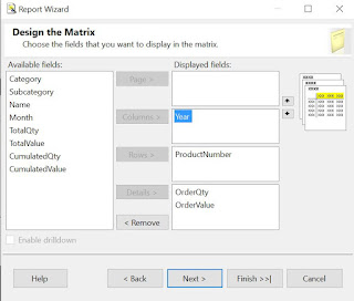
Using the Report Wizard create a new matrix report called "Sales Volume per Product" based on either of the above queries (I considered the second). Within "Design the Matrix" select the attributes as follows:

Design the Matrix

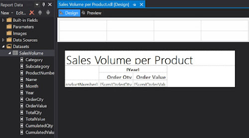
This will create the backbone for our report:

First draft in Design mode

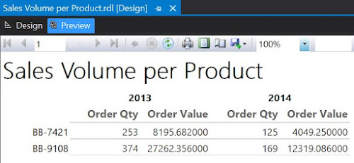
Which is pretty basic, if we consider the output:

First draft in Preview mode

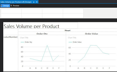
Now, returning in Design mode, right click on the "Sum of OrderQty" cell and from the floating menu select Insert/Chart, while from the list of available charts select Line. Do the same for "Sum of OrderValue". And here's the result:

Second draft in Design mode

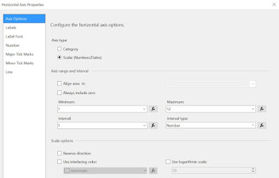
As only one series will be displayed, select the Chart Title and delete the respective label. Delete the Series label as well. When running the report you'll observe that the horizontal axis values are not really appealing. To dix this right click on the respective area and from the floating menu select Horizontal Axis Properties. Within Axis Options section change the Axis type as 'Scalar', enter '1' as Minimum, '12' as Maximum, '1' as Interval and 'Number' as Interval type:

Horizontal Axis Properties

In the same window, within the Labels section select 'Enable auto-fit' and uncheck the "Labels can be offset", respectively the "Labels can be rotated" checkboxes. 

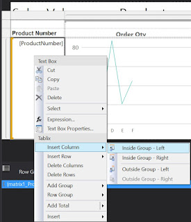
To include the Category, Subcategory and eventually the Product Name, select the Product Number cell, right click on it, and from the floating menu select Insert Column/Inside Group - Left, then select from the Category as attribute:

Inserting a column within the group

Repeat the process to add the Subcategory. Eventually you can add also the Product Name, though for it you'll have to select "Inside Group - Right". 

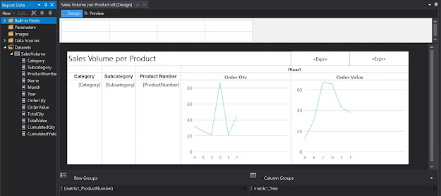
To improve the design, you can add a Page Header and move the report's title into it add a timestamp, respectively a page count textbox, resize the boxes to fit the columns. You can also align the column header values to the center, change the font to 10pt, etc.

Third draft in Design mode

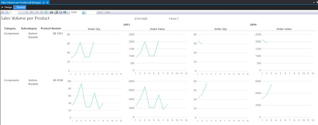
Here's the report in preview mode:

Third draft in Preview mode

One can use the report the way it is, or add the Category and Subcategory as parameters. Similarly, one can use the cumulative values as input for the charts. 

Revamping the Report with Sparklines

Even if the charts allow displaying the scales, the problem with them is that they are too big, which makes it difficult to compare the data across records. One can correct this by using the other types of graphics available in reports, e.g. sparklines. For this make a copy of the report already built, and within the Detail cells select a Sparkine Column instead of a chart:

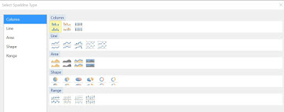
Sparkline types

In comparison with Lines, Column-based representations allow to see how many data points are represented. Because spartklines are more compact as graphic forms, you can resize the cells as follows:

Fourth draft in Design mode

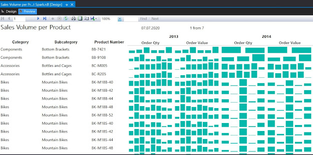
And here's the report in preview mode (the constraints from the source query were removed):

Fourth draft in Preview mode

As can be seen one can easily identify the trends however the volume scale was lost, being impossible to compare which of the Products sold better. One can bring the Total Quantity and Value as display information and sort the dataset from the highest to lowest value. One can even select a top x, to reduce the focus only to the most sold Products.

If the prices remained relatively constant over time, there's actually almost no difference between the graphic displays for Order Quantity, respectively for Order Value. Therefore one can remove one of them (e.g. Order Quantity). Being more compact, sparkline-based representations allow to better use the space, therefore you can add more fields into the report. 

Happy coding!