Power BI: Working with Visual Calculations (Part III: Matrix Tables with Square Numbers as Example)

Introduction

In the previous post I exemplified various operations that can be performed with visual calculations on simple tables based on square numbers. Changing the simple table to a matrix table doesn't bring any benefit. The real benefit comes when one restructures the table to store only a cell per row in a table. 

Data Modelling

For this the Magic5 table can be transformed via the following code, which creates a second table (e.g. M5):

M5 = UNION (
    SUMMARIZECOLUMNS(
     Magic5[Id]
     , Magic5[R]
     , Magic5[Index]
     , Magic5[C1]
     , "Col", "C1"
    )
    , SUMMARIZECOLUMNS(
     Magic5[Id]
     , Magic5[R]
     , Magic5[Index]
     , Magic5[C2]
     , "Col", "C2"
    )
    , SUMMARIZECOLUMNS(
     Magic5[Id]
     , Magic5[R]
     , Magic5[Index]
     , Magic5[C3]
     , "Col", "C3"
    )
    ,  SUMMARIZECOLUMNS(
     Magic5[Id]
     , Magic5[R]
     , Magic5[Index]
     , Magic5[C4]
     , "Col", "C4"
    )
    , SUMMARIZECOLUMNS(
      Magic5[Id]
     , Magic5[R]
     , Magic5[Index]
     , Magic5[C5]
     , "Col", "C5"
    )
)

Once this done, one can add the column [Col] as values for the matrix in a new visual. From now on, all the calculations can be done on copies of this visual. 

Simple Operations

The behavior of the RUNNINGSUM and other functions is different when applied on a matrix table because the formula is applied to every cell of the N*N table, a column with the result being added for each existing column of the matrix.

Moreover, there are four different ways of applying the formula based on the Axis used. ROW calculates the formula by the row within a column:

Run SumByRow(C) = RUNNINGSUM([C], ROWS)

Output:

R	C	Run Sum(C)	C	Run Sum(C)	C	Run Sum(C)	C	Run Sum(C)	C	Run Sum(C)
R1	18	18	25	25	2	2	9	9	11	11
R2	4	22	6	31	13	15	20	29	22	33
R3	15	37	17	48	24	39	1	30	8	41
R4	21	58	3	51	10	49	12	42	19	60
R5	7	65	14	65	16	65	23	65	5	65

By providing COLUMNS as parameter for the Axis makes the calculation run by the column within a row: 

Run SumByCol(C) = RUNNINGSUM([C], COLUMNS)

Output:

R	C	Run Sum(C)	C	Run Sum(C)	C	Run Sum(C)	C	Run Sum(C)	C	Run Sum(C)
R1	18	18	25	43	2	45	9	54	11	65
R2	4	4	6	10	13	23	20	43	22	65
R3	15	15	17	32	24	56	1	57	8	65
R4	21	21	3	24	10	34	12	46	19	65
R5	7	7	14	21	16	37	23	60	5	65

By providing ROW COLUMNS as parameter for the Axis makes the calculation run by the column and then continuing the next column (without resetting the value at the end of the column):

Run SumByRow-Col(C) = RUNNINGSUM([C],ROWS COLUMNS)

Output:

R	C	Run Sum(C)	C	Run Sum(C)	C	Run Sum(C)	C	Run Sum(C)	C	Run Sum(C)
R1	18	18	25	90	2	132	9	204	11	271
R2	4	22	6	96	13	145	20	224	22	293
R3	15	37	17	113	24	169	1	225	8	301
R4	21	58	3	116	10	179	12	237	19	320
R5	7	65	14	130	16	195	23	260	5	325

By providing COLUMNS ROWS as parameter for the Axis makes the calculation run by the row and then continuing the next row (without resetting the value at the end of the column):

Run SumByCol-Row = RUNNINGSUM([C],COLUMNS ROWS)

Output:

R	C	Run Sum(C)	C	Run Sum(C)	C	Run Sum(C)	C	Run Sum(C)	C	Run Sum(C)
R1	18	18	25	43	2	45	9	54	11	65
R2	4	69	6	75	13	88	20	108	22	130
R3	15	145	17	162	24	186	1	187	8	195
R4	21	216	3	219	10	229	12	241	19	260
R5	7	267	14	281	16	297	23	320	5	325

Ranking

RANK can be applied independent of the values, or considering the value with ASC or DESC sorting:

RankByRow = RANK(DENSE,ROWS) -- ranking by row independent of values
RankByRow ASC = RANK(DENSE,ROWS, ORDERBY([C],ASC)) -- ranking by row ascending
RankByRow DESC = RANK(DENSE,ROWS, ORDERBY([C], DESC)) -- ranking by row descending
RankByRow-Col ASC = RANK(DENSE,ROWS COLUMNS, ORDERBY([C],ASC)) -- ranking by row columns ascending
RankByRow-Col DESC = RANK(DENSE,ROWS COLUMNS, ORDERBY([C], DESC)) -- ranking by row columns ascending

[RankByRow-Col ASC] matches the actual numbers from the matrix and is thus useful when sorting any numbers accordingly. 

Differences

Differences can be calculated between any of the cells of the matrix:

DiffToPrevByRow = [C] - PREVIOUS([C])  -- difference to previous record
DiffToPrevByRow* = IF(NOT(IsBlank(PREVIOUS([C]))), [C] - PREVIOUS([C])) -- extended difference to previous record
DiffToPrevByRow-Col = [C] - PREVIOUS([C],, ROWS COLUMNS) -- difference to previous record by ROWS COLUMNS
DiffToFirstByRow = [C] - FIRST([C]) -- difference to first record
DiffToPrevByCol = [C] - FIRST([C], COLUMNS) -- difference to previous record COLUMNS

Ranking = RANK(DENSE, ROWS COLUMNS, ORDERBY([C], ASC)) -- ranking of values by ROWS COLUMNS
OffsetDiffToPrevByRow = [C] - calculate([C], OFFSET(1, ROWS, ORDERBY([Ranking],DESC))) -- difference to the previous record by ROW
OffsetDiffToPrevByRow-Col = [C] - calculate([C], OFFSET(1, ROWS COLUMNS, ORDERBY([Ranking],DESC))) -- difference to the previous record by ROW

Ranking has been introduced to facilitate the calculations based on OFFSET.

The other functions [1] can be applied similarly.

Happy coding!

Previous Post <<||>> Next Post

References:
[1] Microsoft Learn (2024) Power BI: Using visual calculations [preview] (link)

Power BI: Working with Visual Calculations (Part I: Test Drive) [new feature]

Introduction

I recently watched a webcast with Jeroen (Jay) ter Heerdt (see [2]) in which he introduces visual calculations, a type of DAX calculation that's defined and executed directly on a visual [1]. Visual calculations provide an approach of treating a set of data much like an Excel table, allowing to refer to any field available on a visual and write formulas, which simplifies considerably the solutions used currently for ranking records, running averages and other windowing functions. 

The records behind a visual can be mentally represented as a matrix, while the visual calculations can refer to any column from the matrix, allowing to add new columns and include the respective columns in further calculations. Moreover, if a column is used in a formula, it's not recalculated as is the case of measures, which should improve the performance of DAX formulas considerably. 

Currently, one can copy a formula between visuals and if the formula contains fields not available in the targeted visual, they are added as well. Conversely, it's possible to build such a visual, copy it and then replace the dimension on which the analysis is made (e.g. Customer with Product), without being needed to make further changes. Unfortunately, there are also downsides: (1) the calculations are visible only within the visual in which were defined; (2) currently, the visual's data can't be exported if a visual calculation is added; (3) no formatting is supported, etc.

Ranking and Differences

I started to build a solution based on publicly available sales data, which offers a good basis for testing the use of visual calculations. Based on a Power BI visual table made of [Customer Name], [Sales Amount], [Revenue] and [Total Discount], I've added several calculations:

-- percentages
Sales % = 100*DIVIDE([Sales Amount], COLLAPSE([Sales Amount], ROWS))
Revenue % = 100*DIVIDE([Revenue],[Sales Amount])
Discount % = 100*DIVIDE([Total  Discount], [Total  Discount]+[Sales Amount])

-- rankings 
Rank Sales = Rank(DENSE, ORDERBY([Sales Amount], DESC))
Rank Revenue = Rank(DENSE, ORDERBY([Revenue], DESC))

-- differences between consecutive values
Diff. to Prev. Sales = IF([Rank Sales]>1, INDEX([Rank Sales]-1, , ORDERBY([Sales Amount], DESC)) - [Sales Amount] , BLANK())
Diff. to Prev. Rev. = IF([Rank Revenue]>1, INDEX([Rank Revenue]-1, , ORDERBY([Revenue], DESC)) - [Revenue] , BLANK())

Here's the output considered only for the first 10 records sorted by [Sales Amount]:

Customer Name	Sales Amount	Sales %	Revenue	Revenue %	Total Discount	Discount %	Rank Sales	Diff. to Prev. Sales.	Rank Rev.	Diff. to Prev. Rev.
Medline	1058923.78	3.76	307761.99	3.75	126601.02	10.68	1		1
Ei	707663.21	2.51	229866.98	2.8	95124.09	11.85	2	351260.57	2	77895.01
Elorac, Corp	702911.91	2.49	209078.76	2.55	83192.39	10.58	3	4751.3	6	20788.22
Sundial	694918.98	2.47	213362.1	2.6	78401.72	10.14	4	7992.93	4	-4283.34
OUR Ltd	691687.4	2.45	196396.26	2.4	78732.2	10.22	5	3231.58	10	16965.84
Eminence Corp	681612.78	2.42	213002.78	2.6	86904.03	11.31	6	10074.62	5	-16606.52
Apotheca, Ltd	667283.99	2.37	157435.56	1.92	101453.91	13.2	7	14328.79	31	55567.22
Rochester Ltd	662943.9	2.35	224918.2	2.74	81158.11	10.91	8	4340.09	3	-67482.64
ETUDE Ltd	658370.48	2.34	205432.79	2.51	89322.72	11.95	9	4573.42	9	19485.41
Llorens Ltd	646779.31	2.29	206567.4	2.52	82897.59	11.36	10	11591.17	8	-1134.61

Comments:
1) One could use [Total Amount] = [Total  Discount]+[Sales Amount] as a separate column.
2) The [Rank Sales] is different from the [Rank Rev.] because of the discount applied.
3) In the last two formulas a blank was considered for the first item from the ranking.
4) It's not possible to control when the totals should be displayed, however one can change the color for the not needed total to match the background.

Visualizing Differences 

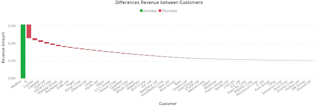
Once the formulas are added, one can hide the basis columns and visualize the data as needed. To obtain the below chart I copied the visual and changed the column as follows:

Diff. to Prev. Rev. = IF([Rank Revenue]>1, [Revenue]- INDEX([Rank Revenue]-1, , ORDERBY([Revenue], DESC)) , [Revenue]) -- modified column

Comments:

1) Instead of showing the full revenue, the chart shows only the differences from the highest revenue, where the column in green is the highest revenue, while the columns in red are the differences of the current customer's revenue to the previous customer, as the data are sorted by the highest revenue. At least in this case it results in a lower data-ink ratio (see Tufte).

2) The values are sorted by the [Revenue] descending. 

3) Unfortunately, it's not possible to change the names from the legend.

Simple Moving Averages (SMAs)

Based on the [Sales Amount], [Revenue] and [Month] one can add the following DAX formulas to the table for calculating the SMA:

Sales Amount (SMA) = MOVINGAVERAGE([Sales Amount],6)
Revenue (SMA) = MOVINGAVERAGE([Revenue],6)

The chart becomes:

Comments:

1) Unfortunately, the formula can't project the values into the feature, at least not without the proper dates.
2) "Show items with not data" feature seems to be disabled when visual calculations are used.

3) The SMA was created via a template formula. Similarly, calculating a running sum is reduced to applying a formula:

Running Sales Amount = RUNNINGSUM([Sales Amount])

Wrap Up

It's easier to start with a table for the visual, construct the needed formulas and then use the proper visual while eliminating the not needed fields. 

The feature is still in public preview and changes can still occur. Unfortunately, there's still no information available on the general availability date. From the first tests, it provides considerable power with a minimum of effort, which is great! I don't want to think how long I would have needed to obtain the same results without it!

Happy coding!

Previous Post <<||>> Next Post

References: 
[1] Microsoft Learn (2024) Power BI: Using visual calculations [preview] (link)
[2] SSBI Central (2024) Visual Calculations - Making DAX easier, with Jeroen ter Heerdt (link)

SQL Reloaded: The WINDOW Clause in SQL Server 2022 (Part III: Ranking)

In two previous posts I shown how to use the newly introduced WINDOW clause in SQL Server 2022 for simple aggregations, respectively running totals, by providing some historical context concerning what it took to do the same simple aggregations as SUM or AVG within previous versions of SQL Server. Let's look at another scenario based on the previously created Sales.vSalesOrders view - ranking records within a partition. 

There are 4 ranking functions that work across partitions: Row_Number, Rank, Dense_Rank and NTile. However, in SQL Server 2000 only Row_Number could be easily implemented, and this only if there is a unique identifier (or one needed to create one on the fly):

-- ranking based on correlated subquery (SQL Server 2000+)
SELECT SOL.SalesOrderId 
, SOL.ProductId
, SOL.OrderDate
, SOL.[Year]
, SOL.[Month]
, SOL.OrderQty
, (-- correlated subquery
  SELECT count(SRT.SalesOrderId)
  FROM Sales.vSalesOrders SRT
  WHERE SRT.ProductId = SOL.ProductId 
    AND SRT.[Year] = SOL.[Year]
	AND SRT.[Month] = SOL.[Month]
    AND SRT.SalesOrderId <= SOL.SalesOrderId
   ) RowNumberByDate
FROM Sales.vSalesOrders SOL
WHERE SOL.ProductId IN (745)
  AND SOL.[Year] = 2012
  AND SOL.[Month] BETWEEN 1 AND 3
ORDER BY SOL.[Year]
, SOL.[Month]
, SOL.OrderDate ASC

As alternative for implementing the other ranking functions, one could use procedural language for looping, though this approach was not recommendable given the performance concerns.

SQL Server 2005 introduced all 4 ranking functions, as they are in use also today:

-- ranking functions (SQL Server 2005+)
SELECT SOL.SalesOrderId 
, SOL.ProductId
, SOL.OrderDate
, SOL.[Year]
, SOL.[Month]
, SOL.OrderQty
-- rankings
, Row_Number() OVER (PARTITION BY SOL.ProductId, SOL.[Year], SOL.[Month] ORDER BY SOL.OrderQty DESC) RowNumberQty
, Rank() OVER (PARTITION BY SOL.ProductId, SOL.[Year], SOL.[Month] ORDER BY SOL.OrderQty DESC) AS RankQty
, Dense_Rank() OVER (PARTITION BY SOL.ProductId, SOL.[Year], SOL.[Month] ORDER BY SOL.OrderQty DESC) AS DenseRankQty
, NTile(4) OVER (PARTITION BY SOL.ProductId, SOL.[Year], SOL.[Month] ORDER BY SOL.OrderQty DESC) AS NTileQty
FROM Sales.vSalesOrders SOL
WHERE SOL.ProductId IN (745)
  AND SOL.[Year] = 2012
  AND SOL.[Month] BETWEEN 1 AND 3
ORDER BY SOL.[Year]
, SOL.[Month]
, SOL.OrderQty DESC

Now, in SQL Server 2022 the WINDOW clause allows simplifying the query as follows by defining the partition only once:

-- ranking functions (SQL Server 2022+)
SELECT SOL.SalesOrderId 
, SOL.ProductId
, SOL.OrderDate
, SOL.[Year]
, SOL.[Month]
, SOL.OrderQty
-- rankings

, Row_Number() OVER SalesByMonth AS RowNumberQty
, Rank() OVER SalesByMonth AS RankQty
, Dense_Rank() OVER SalesByMonth AS DenseRankQty
, NTile(4) OVER SalesByMonth AS NTileQty
FROM Sales.vSalesOrders SOL
WHERE SOL.ProductId IN (745)
  AND SOL.[Year] = 2012
  AND SOL.[Month] BETWEEN 1 AND 3
WINDOW SalesByMonth AS (PARTITION BY SOL.ProductId, SOL.[Year], SOL.[Month] ORDER BY SOL.OrderQty DESC)
ORDER BY SOL.[Year]
, SOL.[Month]
, SOL.OrderQty DESC

Forward (and backward) referencing of one window into the other can be used with ranking functions as well:

 

-- ranking functions with ascending/descending sorting (SQL Server 2022+)
SELECT SOL.SalesOrderId 
, SOL.ProductId
, SOL.OrderDate
, SOL.[Year]
, SOL.[Month]
, SOL.OrderQty
-- rankings (descending)
, Row_Number() OVER SalesByMonthSortedDESC AS DescRowNumberQty
, Rank() OVER SalesByMonthSortedDESC AS DescRankQty
, Dense_Rank() OVER SalesByMonthSortedDESC AS DescDenseRankQty
, NTile(4) OVER SalesByMonthSortedDESC AS DescNTileQty
-- rankings (ascending)
, Row_Number() OVER SalesByMonthSortedASC AS AscRowNumberQty
, Rank() OVER SalesByMonthSortedASC AS AscRankQty
, Dense_Rank() OVER SalesByMonthSortedASC AS AscDenseRankQty
, NTile(4) OVER SalesByMonthSortedASC AS AscNTileQty
FROM Sales.vSalesOrders SOL
WHERE SOL.ProductId IN (745)
  AND SOL.[Year] = 2012
  AND SOL.[Month] BETWEEN 1 AND 3
WINDOW SalesByMonth AS (PARTITION BY SOL.ProductId, SOL.[Year], SOL.[Month])
, SalesByMonthSortedDESC AS (SalesByMonth ORDER BY SOL.OrderQty DESC)
, SalesByMonthSortedASC AS (SalesByMonth ORDER BY SOL.OrderQty ASC)
ORDER BY SOL.[Year]
, SOL.[Month]
, SOL.OrderQty DESC

Happy coding!

SSRS (& Paginated Reports): Ranking Rows in Reports

Introduction

In almost all the reports I built, unless it was explicitly requested no to, I prefer adding a running number (aka ranking) for each record contained into the report, while providing different background colors for consecutive rows. The ranking allows easily identify a record when discussing about it within the report or extracts, while the different background colors allow differentiating between two records while following the values which scrolling horizontally. The logic for the background color can be based on two (or more) colors using the ranking as basis.

Tabular Reports

In a tabular report the RowNumber() function is the straightforward way for providing a ranking. One just needs to add a column into the report before the other columns, giving a meaningful name (e.g. RankingNo) and provide the following formula within its Expression:
= RowNumber(Nothing)

When 'Nothing' is provided as parameter, the ranking is performed across all the report. If is needed to restrict the Ranking only to a grouping (e.g. Category), then group's name needs to be provided as parameter:
= RowNumber("Category")

Matrix Reports

Unfortunately, in a matrix report based on aggregation of raw data the RowNumber() function stops working, the values shown being incorrect. The solution I use to solve this is based on the custom GetRank() VB function:

Dim Rank as Integer = 0
Dim LastValue as String = ""

Function GetRank(group as string) as integer
if group <> LastValue then
       Rank = Rank + 1
       LastValue = group
end if

return Rank
end function

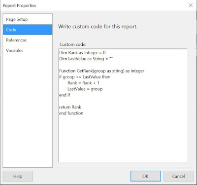
The function compares the values provided in the call against a global scope LastValue text value. If the values are different, then a global scope Rank value is incremented by1, while the LastValue is initialized to the new value, otherwise the values remaining the same. The logic is basic also for a non-programmer.

The above code needs to be added into the Code section of Report's Properties for the function to be available:

Adding the code in Report Properties

Once the function added, a new column should be added similarly as for a tabular report,  providing the following code within its Expression in exchange:
=Code.GetRank(Fields!ProductNumber.Value)

Note:
As it seems, on the version of Reporting Services Extension I use, the function has only a page scope, the value being reset after each page. However when exporting the data with Excel the ranking is applied to the whole dataset.

Providing Alternate Colors

Independently of the report type, one can provide an alternate color for table's rows by selecting the row with the data and adding the following expression into the BackaroundColor property:
=Iif(ReportItems!RankingNo.Value Mod 2, "White", "LightSteelBlue")

Notes:
1) For a tabular report the cost of calling the RowNumber function instead of referring to the RankingNo cell is relatively small. One can write it also like this:
=llf(RowNumber(Nothing) Mod 2 = 0, "White", "LightSteelBlue")

Power BI Paginated Reports

The pieces of code considered above can be used also in Power BI Paginated Reports. Even if there's no functionality for adding custom code in the standard UI, one can make changes to the rdl file in Visual Studio or even in Notepad. For example, one can add the code within the "Code" tag at the end of the file before the closing tag for the report:

<Code>Dim Rank as Integer = 0
Dim LastValue as String = ""
Dim Concatenation = ""

Function GetRank(group as string) as integer
if group <> LastValue then
       Rank = Rank + 1
       LastValue = group
end if

Concatenation = Concatenation & vbCrLf & Rank & "/" & group &amp; "/" & LastValue
return Rank
end function</Code>
</Report>

Note:

One can consider using a pipeline "|" instead of a forward slash.

SQL Server New Features: Window Functions

Introduction

     In the past, in the absence or in parallel with other techniques, aggregate functions proved to be quite useful in order to solve several types of problems that involve the retrieval of first/last record or the display of details together with averages and other aggregates. Typically their use involves two or more joins between a dataset and an aggregation based on the same dataset or a subset of it. An aggregation can involve one or more columns that make the object of analysis. Sometimes it might be needed multiple such aggregations based on different sets of columns. Each such aggregation involves at least a join. Such queries can become quite complex, though they were a price to pay in order to solve such problems.

Partitions

     The introduction of analytic functions in Oracle and of window functions, a similar concept, in SQL Server, allowed the approach of such problems from a different simplified perspective. Central to this feature it’s the partition (of a dataset), its meaning being same as of mathematical partition of a set, defined as a division of a set into non-overlapping and non-empty parts that cover the whole initial set. The introduction of partitions it’s not necessarily something new, as the columns used in a GROUP BY clause determines (implicitly) a partition in a dataset. The difference in analytic/window functions is that the partition is defined explicitly inline together with a ranking or average function evaluated within a partition. If the concept of partition is difficult to grasp, let’s look at the result-set based on two Products (the examples are based on AdventureWorks database):
 

-- Price Details for 2 Products 
SELECT A.ProductID  
, A.StartDate 
, A.EndDate 
, A.StandardCost  
FROM [Production].[ProductCostHistory] A 
WHERE A.ProductID IN (707, 708) 
ORDER BY A.ProductID 
, A.StartDate 

   In this case a partition is “created” based on the first Product (ProductId = 707), while a second partition is based on the second Product (ProductId = 708). As a parenthesis, another partitioning could be created based on ProductId and StartDate; considering that the two attributes are a key in the table, this will partition the dataset in partitions of 1 record (each partition will have exactly one record).

Details and Averages

     In order to exemplify the use of simple versus window aggregate functions, let’s consider a problem in which is needed to display Standard Price details together with the Average Standard Price for each ProductId. When a GROUP BY clause is applied in order to retrieve the Average Standard Cost, the query is written under the form: 

-- Average Price for 2 Products 
SELECT A.ProductID  
, AVG(A.StandardCost) AverageStandardCost 
FROM [Production].[ProductCostHistory] A 
WHERE A.ProductID IN (707, 708) 
GROUPBY A.ProductID  
ORDERBY A.ProductID 

 

    In order to retrieve the details, the query can be written with the help of a FULL JOIN as follows:

-- Price Details with Average Price for 2 Products - using JOINs 
SELECT A.ProductID  
, A.StartDate 
, A.EndDate 
, A.StandardCost 
, B.AverageStandardCost 
, A.StandardCost - B.AverageStandardCost DiffStandardCost 
FROM [Production].[ProductCostHistory] A    
  JOIN ( -- average price        
    SELECT A.ProductID         
    , AVG(A.StandardCost) AverageStandardCost         
    FROM [Production].[ProductCostHistory] A        
    WHERE A.ProductID IN (707, 708)        
    GROUP BY A.ProductID      
) B  
    ON A.ProductID = B.ProductID 
WHERE A.ProductID IN (707, 708) 
ORDERBY A.ProductID 
, A.StartDate 

    

    As pointed above the partition is defined by ProductId. The same query written with window functions becomes:

-- Price Details with Average Price for 2 Products - using AVG window function 
SELECT A.ProductID  
, A.StartDate 
, A.EndDate 
, A.StandardCost 
, AVG(A.StandardCost) OVER(PARTITION BY A.ProductID) AverageStandardCost 
, A.StandardCost - AVG(A.StandardCost) OVER(PARTITION BY A.ProductID) DiffStandardCost 
FROM [Production].[ProductCostHistory] A 
WHERE A.ProductID IN (707, 708) 
ORDER BY A.ProductID 
, A.StartDate 

    As can be seen, in the second example, the AVG function is defined using the OVER clause with PartitionId as partition. Even more, the function is used in a formula to calculate the Difference Standard Cost. More complex formulas can be written making use of multiple window functions.  

The Last Record

     Let’s consider the problem of retrieving the nth record. Because with aggregate functions is easier to retrieve the first or last record, let’s consider that is needed to retrieve the last Standard Price for each ProductId. The aggregate function helps to retrieve the greatest Start Date, which farther helps to retrieve the record containing the Last Standard Price.

-- Last Price Details for 2 Products - using JOINs 
SELECT A.ProductID  
, A.StartDate 
, A.EndDate 
, A.StandardCost 
FROM [Production].[ProductCostHistory] A  
    JOIN ( -- average price          
    SELECT A.ProductID          
    , Max(A.StartDate) LastStartDate          
    FROM [Production].[ProductCostHistory] A          
    WHERE A.ProductID IN (707, 708)          
    GROUP BY A.ProductID      
) B      
   ON A.ProductID = B.ProductID  
  AND A.StartDate = B.LastStartDate 
WHERE A.ProductID IN (707, 708) 
ORDERBY A.ProductID 
,A.StartDate 

  

With window functions the query can be rewritten as follows:

-- Last Price Details for 2 Products - using AVG window function 
SELECT * 
FROM (-- ordered prices      
    SELECT A.ProductID      
    , A.StartDate      
    , A.EndDate      
    , A.StandardCost      
    , RANK() OVER(PARTITION BY A.ProductID ORDER BY A.StartDate DESC) Ranking      
    FROM [Production].[ProductCostHistory] A     
    WHERE A.ProductID IN (707, 708) 
  ) A 
WHERE Ranking = 1 
ORDER BY A.ProductID 
, A.StartDate 

  

   As can be seen, in order to retrieve the Last Standard Price, was considered the RANK function, the results being ordered descending by StartDate. Thus, the Last Standard Price will be always positioned on the first record. Because window functions can’t be used in WHERE clauses, it’s needed to encapsulate the initial logic in a subquery. Similarly could be retrieved the First Standard Price, this time ordering ascending the StartDate. The last query can be easily modified to retrieve the nth records (this can prove to be more difficult with simple average functions), the first/last nth records.

Conclusion

    Without going too deep into details, I shown above two representative scenarios in which solutions based on average functions could be simplified by using window functions. In theory the window functions provide greater flexibility but they have their own trade offs too. In the next posts I will attempt to further detail their use, especially in the context of Statistics.