Showing posts with label AdventureWorks. Show all posts

25 December 2024

💎🏭SQL Reloaded: Number of Records IV (via sys.partitions)

To get the exact number of records in a table one can use the COUNT (see post) or the more recent COUNT_BIG function, though for big tables this can be an inefficient operation for the database engine:

-- number of records via COUNT
SELECT count(*) row_count
FROM SalesLT.Product

Moreover, sometimes the operation needs to be repeated for a number of tables, e.g. dropdown tables in Dynamics 365 for Finance and Operations (D365 F&O). Writing the query as a UNION allows to export the data as a single table and do comparisons (e.g. in Excel). The same approach can be used also when multiple columns are used for grouping, though one must account for the additional columns in the other subqueries. However, the more tables are involved, the more difficult it becomes to maintain the query over time. 
 
-- number of records via COUNT for multiple tables
SELECT 'SalesLT.Product' table_name
, count(*) row_count
FROM SalesLT.Product
UNION ALL
SELECT 'SalesLT.ProductDescription' table_name
, count(*) row_count
FROM SalesLT.ProductDescription
UNION ALL
SELECT 'SalesLT.ProductModel' table_name
, count(*) row_count
FROM SalesLT.ProductModel

There are many scenarios in which it's needed to get an approximate of the number of records available in a table and doing a record count might prove to be too expensive. For a quick and dirty solution one can use the sys.partitions DMV  instead:

-- number of records via DMV for single object
SELECT object_id
, OBJECT_NAME(object_id) object_name
, OBJECT_SCHEMA_NAME(object_id) schema_name
, SUM(Rows) AS row_count
, data_compression_desc AS compression_type
, COUNT(*) partitions_count
FROM sys.partitions 
WHERE index_id < 2 --ignore the partitions from the non-clustered index if any
  AND OBJECT_ID('SalesLT.Product') = object_id
GROUP BY object_id
, data_compression_desc
ORDER BY row_count DESC;

The query is based on sys.partitions table [1] which contains a row for each partition of all the tables and most types of indexes in the database. The documentation mentions that "rows" indicates the approximate number of rows in the considered partition.

Alternatively, one can bring more tables into the query to extend its range of applicability. 

-- number of records via DMVs
SELECT S.name + '.' + T.name SearchName
, S.Name SchemaName
, T.name TableName
, P.row_count
, P.compression_type
, P.partitions_count
FROM sys.tables T
     LEFT JOIN (
        SELECT object_id
        , SUM(Rows) AS row_count
        , data_compression_desc AS compression_type
        , COUNT(*) partitions_count
        FROM sys.partitions 
        WHERE index_id < 2 --ignore the partitions from the non-clustered index if any
        --AND OBJECT_ID('SalesLT.Product') = object_id
        GROUP BY object_id
        , data_compression_desc
     ) P
    ON T.object_id = P.object_id
     JOIN sys.schemas as S
	   on S.schema_id = T.schema_id
WHERE S.Name = 'SalesLT'
  AND T.Name LIKE 'Product%'
ORDER BY row_count DESC;

The data can be exported regularly to give an idea how tables' cardinality changes over time. One can find this useful as part of the loading process in data warehouses or other solutions (e.g. data migrations). 

By using a FULL JOIN instead of a LEFT JOIN one can retrieve only the tables that have records. 

One should consider only the tables in scope, and eventually remove the records associated with the system objects (e.g. sys or information_schema upon case).

 -- constraints to be added in the WHERE clause to remove the records related to system objects
 AND OBJECT_NAME(object_id) NOT LIKE 'sys%'
 AND OBJECT_NAME(object_id) NOT LIKE 'queue_%' 
 AND OBJECT_NAME(object_id) NOT LIKE 'filestream_tombstone%' 

There are also scenarios in which the count is needed only for a subset of the data. It's the case of D365 F&O (in which the number of records is needed by DataAreaId (aka company) or another field. A solution can be built using the sp_MSForEachTable stored procedure (see the last query from this post) and a cursor.

Notes:
The code used in this post is available also in the GitHub repository.

Happy coding and Merry Christmas!

Previous Post <<||>> Next Post

Resources:
[1] Microsoft Learn (2024) sys.partitions (Transact-SQL) [link]
[2] Microsoft Learn (2024) COUNT_BIG (Transact-SQL) [link]

21 December 2024

💎🏭SQL Reloaded: Microsoft Fabric's SQL Databases (Part I: Creating a View) [new feature]

At this year's Ignite conference it was announced that SQL databases are available now in Fabric in public preview (see SQL Databases for OLTP scenarios, [1]). To test the functionality one can import the SalesLT database in a newly created empty database, which made available several tables:
 
-- tables from SalesLT schema (queries should be run individually)
SELECT TOP 100 * FROM SalesLT.Address
SELECT TOP 100 * FROM SalesLT.Customer
SELECT TOP 100 * FROM SalesLT.CustomerAddress
SELECT TOP 100 * FROM SalesLT.Product ITM 
SELECT TOP 100 * FROM SalesLT.ProductCategory
SELECT TOP 100 * FROM SalesLT.ProductDescription 
SELECT TOP 100 * FROM SalesLT.ProductModel  
SELECT TOP 100 * FROM SalesLT.ProductModelProductDescription 
SELECT TOP 100 * FROM SalesLT.SalesOrderDetail
SELECT TOP 100 * FROM SalesLT.SalesOrderHeader

The schema seems to be slightly different than the schemas used in previous tests made in SQL Server, though with a few minor changes - mainly removing the fields not available - one can create the below view:
 
-- drop the view (cleaning step)
-- DROP VIEW IF EXISTS SalesLT.vProducts 

-- create the view
CREATE OR ALTER VIEW SalesLT.vProducts
-- Products (view) 
AS 
SELECT ITM.ProductID 
, ITM.ProductCategoryID 
, PPS.ParentProductCategoryID 
, ITM.ProductModelID 
, ITM.Name ProductName 
, ITM.ProductNumber 
, PPM.Name ProductModel 
, PPS.Name ProductSubcategory 
, PPC.Name ProductCategory  
, ITM.Color 
, ITM.StandardCost 
, ITM.ListPrice 
, ITM.Size 
, ITM.Weight 
, ITM.SellStartDate 
, ITM.SellEndDate 
, ITM.DiscontinuedDate 
, ITM.ModifiedDate 
FROM SalesLT.Product ITM 
     JOIN SalesLT.ProductModel PPM 
       ON ITM.ProductModelID = PPM.ProductModelID 
     JOIN SalesLT.ProductCategory PPS 
        ON ITM.ProductCategoryID = PPS.ProductCategoryID 
         JOIN SalesLT.ProductCategory PPC 
            ON PPS.ParentProductCategoryID = PPC.ProductCategoryID

-- review the data
SELECT top 100 *
FROM SalesLT.vProducts

In the view were used FULL JOINs presuming thus that a value was provided for each record. It's always a good idea to test the presumptions when creating the queries, and eventually check from time to time whether something changed. In some cases it's a good idea to always use LEFT JOINs, though this might have impact on performance and probably other consequences as well.
 
-- check if all models are available
SELECT top 100 ITM.*
FROM SalesLT.Product ITM 
    LEFT JOIN SalesLT.ProductModel PPM 
       ON ITM.ProductModelID = PPM.ProductModelID 
WHERE PPM.ProductModelID IS NULL

-- check if all models are available
SELECT top 100 ITM.*
FROM SalesLT.Product ITM 
    LEFT JOIN SalesLT.ProductCategory PPS 
        ON ITM.ProductCategoryID = PPS.ProductCategoryID 
WHERE PPS.ProductCategoryID IS NULL

-- check if all categories are available
SELECT PPS.*
FROM SalesLT.ProductCategory PPS 
     LEFT JOIN SalesLT.ProductCategory PPC 
       ON PPS.ParentProductCategoryID = PPC.ProductCategoryID
WHERE PPC.ProductCategoryID IS NULL

Because the Product categories have an hierarchical structure, it's a good idea to check the hierarchy as well:
 
-- check the hierarchical structure 
SELECT PPS.ProductCategoryId 
, PPS.ParentProductCategoryId 
, PPS.Name ProductCategory
, PPC.Name ParentProductCategory
FROM SalesLT.ProductCategory PPS 
     LEFT JOIN SalesLT.ProductCategory PPC 
       ON PPS.ParentProductCategoryID = PPC.ProductCategoryID
--WHERE PPC.ProductCategoryID IS NULL
ORDER BY IsNull(PPC.Name, PPS.Name)

This last query can be consolidated in its own view and the previous view changed, if needed.

One can then save all the code as a file. 
Except some small glitches in the editor, everything went smoothly. 

Notes:
1) One can suppose that many or most of the queries created in the previous versions of SQL Server work also in SQL databases. The future and revised posts on such topics are labelled under sql database.
2) During the various tests I got the following error message when trying to create a table:
"The external policy action 'Microsoft.Sql/Sqlservers/Databases/Schemas/Tables/Create' was denied on the requested resource."
At least in my case all I had to do was to select "SQL Database" instead of "SQL analytics endpoint" in the web editor. Check the top right dropdown below your user information.
[3] For a full least of the available features see [2].

Happy coding!

Previous Post <<||>> Next Post

References:
[1] Microsoft Learn (2024) SQL database in Microsoft Fabric (Preview) [link]
[2] Microsoft Learn (2024) Features comparison: Azure SQL Database and SQL database in Microsoft Fabric (preview) [link]

05 April 2024

💎SQL Reloaded: SQL Antipatterns (Part I: JOINs, UNIONs & DISTINCT)

Introduction

SQL antipatterns refer in general to common mistakes made when developing SQL code, though the term can refer also to situations in which even if the code is syntactically and logically correct, it's either suboptimal, unclear or even incorrect. Therefore "mistake" can cover a wide range of scenarios, some that can be ignored, while others need to be addressed accordingly. 

In this post I consider a few antipatterns observed especially in data warehouses (DWHs). Let's look at the below code created to exemplify several scenarios:

-- Products in open orders (initial query)
SELECT DISTINCT ITM.ProductId                                   -- (1) use of DISTINCT
, ITM.ProductNumber
, ITM.Name 
, ITM.Color 
, ITM.Style 
, ITM.Size
FROM Production.Product ITM
    LEFT JOIN (							-- (5) use of JOIN instead of EXISTS
	-- Open Purchase orders 
	SELECT DISTINCT POL.ProductId
	, 'POs' Source                                          -- (7) use columns not needed in output
	FROM Purchasing.PurchaseOrderDetail POL                 
	     LEFT JOIN Purchasing.PurchaseOrderHeader POH       -- (2) use of LEFT JOIN instead of FULL JOIN
		  ON POL.PurchaseOrderID = POH.PurchaseOrderID
	WHERE POH.Status = 1 -- pending 
	UNION					                -- (3) use of UNION
	-- Open Sales orders 
	SELECT DISTINCT SOL.ProductId
	, 'SOs' Source
	FROM Sales.SalesOrderDetail SOL
	    LEFT JOIN Sales.SalesOrderHeader SOH
		  ON SOL.SalesOrderID = SOH.SalesOrderID
	WHERE SOH.Status = 1 -- in process		        -- (4) use of OR instead of IN
	   OR SOH.Status = 2 -- approved
	) DAT
	ON ITM.ProductID = DAT.ProductID
WHERE DAT.ProductID IS NOT NULL 
ORDER BY ITM.ProductNumber			                -- (6) using too many columns in ORDER BY
, ITM.Name 
, ITM.Color 
, ITM.Style 
, ITM.Size

(1) Use of DISTINCT 

DISTINCT is a dirty way to remove the duplicates from a dataset. Sometimes it makes sense to use it to check something fast, though it should be avoided into code intended for a production environment because it can lead to unexpected behavior especially when selecting all the columns using the "*" (SELECT DISTINCT *).

I saw tools and developers adding a DISTINCT in almost each step, independently on whether it was necessary or not. One can thus but wonder whether the DISTINCT was added to fix a bigger issue with the data in the DWH, to remove special duplicates imposed by the logic or just as poor practice. Unfortunately, when it's used frequently, it can become challenging to investigate its use and discover the actual issues from the DWH.

There are several approaches to eliminate DISTINCTs from the code: GROUP BY, ranking functions or upon case also code rewrites.

(2)  Use of LEFT JOIN Instead of FULL JOIN

When refreshing a DWH there can be the case that related data are out of synch. It would be the case of Purchase or Sales orders where the headers and lines are out of synch, headers existing without lines and/or vice versa. A common practice is to use a FULL JOIN and thus to eliminate such exceptions, though there are also entitled uses of a LEFT JOIN. This antipattern resumes however to the cases in which logically should be used a FULL JOIN, though a LEFT JOIN is used instead.

In the above example there are two distinct occurrences of this pattern: the relationship between the header and lines in the inner query, respectively the LEFT JOIN with a NOT NULL constraint in the outer query. The latter use is useful when during testing one wants to see all the Products, though bringing this further into production may rise some eyebrows even if it's not necessarily wrong. Anyway, the database engine should be smart enough to recognize such a scenario. However, for the header vs lines case, upon case the plan generated might be suboptimal. 

One of the best practices when writing SQL queries is to state one's intent clearly in what the logic concerns. Using a LEFT JOIN instead of a FULL JOIN can make people raise questions about the actual need. When the need is not properly documented, some developer may even go and change the joins. There can be for example business cases that are not cover by the current data, but as soon as case appears it will lead to incorrect logic!

Similarly, splitting a piece of logic into two or more steps unnecessarily can create confusion. There can be however also entitled s situations (e.g. query optimization), which ideally should be documented.

(3) Use of UNION

When a UNION is used, the values returned by the first query will be checked against the values of the second query, and thus unnecessary comparisons occur even if they are not needed. This depends also on the business context, which might not be easily to identify from the query (especially when the reviewer doesn't know the business case). 

The misuse of a UNION will not make a big difference when the volume of data is small, though the more data are processed by the query, the higher the impact. 

Besides the proper use of the UNION, there are also situations in which a query rewrite can eliminate the need for a UNION (see the rewritten query below).

(4) use of OR instead of IN

One can occasionally find queries in which a OR was used for 10 to 50 distinct values as in the example above. Even if the database engine generate in both cases the same query plan, it's easier to read and maintain a query that used IN. However, if the number of values go beyond a certain value, other techniques should be used to improve the performance.

The only benefit I see for a OR is to document meaning's values or remove during testing one of the values, especially when the list is a selection coming from the user. Frankly, it's not the appropriate way for documenting logic (even if I'm doing it sometimes in ad-hoc queries).

There's a more extreme scenario in which distinct subqueries are written for each or a set of ORs (e.g. the distinction between open vs closed vs. invoices orders), which can make sense sometimes (e.g. the logic is completely different). Therefore, an antipattern can be dependent also of the context or use case. 

(5) use of JOIN instead of EXISTS

When there are no values returned from the subquery, quite often it makes sense to the EXISTS or not EXISTS operators in the queries (see the rewritten query below). This might not be indicated however for distributed environments like serverless SQL pool in which the distribution of the processing across multiple tasks might benefit when the pieces of the logic distributed don't require heavy reshuffles. 

(6) Using too Many Columns in ORDER BY

The columns specified in an ORDER BY clause need to make sense, otherwise they just add extra burden on the database engine, at least from the perspective of the checks that need to be performed. In the above query, at least the Name doesn't make sense.

It helps also if the columns can use existing indexes, though this depends also on query specifics. 

Another antipattern scenario not exemplified above is the use of ordinals to refer to the columns, which should be avoided in production environments (because the order of the columns can be changed accidentally or even :

-- using ordinals instead of number columns (not recommended)
SELECT ITM.ProductId                                  
, ITM.ProductNumber
, ITM.Name 
, ITM.Color 
, ITM.Style 
, ITM.Size
FROM Production.Product ITM                           
ORDER BY 2, 4, 5, 6

(7) Use Columns Not  Needed in Output

Besides the fact that each column included unnecessarily in the query can increase the size of the data processed (unless the database engine is smart to remove them), there can be also performance issues and/or optimizations involved. For example, if all the other columns are part of a covering index, the database engine might opt for a suboptimal index compared to the case in which the unnecessary columns are removed. 

Conversely, some columns are helpful to troubleshoot the logic (and that's why the Source column was considered) even if they aren't considered in the final output or the logic. It doesn't make sense to bring the query version with the respective fields into production, even if this would mean to have maybe a second version of the query used only for troubleshooting needs. Commenting the unnecessary columns could be a better choice, even if it's not recommended in general as too many such comments can obfuscate the case. 

Rewriting the Query

With the above input the query can be rewritten as follows:

-- Products in open orders (modified query)
SELECT ITM.ProductId                                  
, ITM.ProductNumber
, ITM.Name 
, ITM.Color 
, ITM.Style 
, ITM.Size
FROM Production.Product ITM
WHERE EXISTS (										            
	-- Open Purchase orders 
	SELECT POL.ProductId
	FROM Purchasing.PurchaseOrderDetail POL                 
	     JOIN Purchasing.PurchaseOrderHeader POH      
		  ON POL.PurchaseOrderID = POH.PurchaseOrderID
	WHERE POH.Status = 1 
	  AND ITM.ProductID = POL.ProductID
	)
 OR EXISTS (				                                    
	-- Open Sales orders 
	SELECT SOL.ProductId
	FROM Sales.SalesOrderDetail SOL
	     JOIN Sales.SalesOrderHeader SOH
		  ON SOL.SalesOrderID = SOH.SalesOrderID
	WHERE SOH.Status IN (1, 2)
	  AND ITM.ProductID = SOL.ProductID
	)	                           
ORDER BY ITM.ProductNumber			                           
, ITM.Color 
, ITM.Style 
, ITM.Size

Please note that in general to each rule there are also exceptions which should be considered against one's common sense. When the benefit of addressing an antipattern is neglectable compared with the effort involved and the logic doesn't create any issues, probably it's better to let the code as it. One can still reconsider the antipatterns later with the next refactoring opportunity. 

There are zealous data professionals who treat minor inconveniences (e.g. not using upper case for SQL reserved words, alternate code formatting, alternative writing of words, especially function names, different indentation, the use of "--" for commenting within a query, etc.) as antipatterns. Use your common sense and evaluate the effort against the benefits or risks and, not less important, be patient with others' mistakes!

Happy coding!

Previous Post <<||>> Next Post
07 July 2020

🪄SSRS (& Paginated Reports): First Steps (Part V: Small Multiples & Sparklines) )

Introduction 

Using a single chart to display multiple series in SQL Server Reporting Services (SSRS) or any other reporting tool works well when the number of series is somehow manageable - usually being enough to display 2-10 series within the same chart. The more series one adds, the more complicated will be for users to read the chart. One has the choice to find either
-  a level of detail (e.g. Category) which, when grouping the data, leads to a number of manageable series,
-  compare the data within a certain grouping (e.g. Category),
-  displaying the individual trends (e.g. for each Product). 

Let's consider the last choice. The report from this post will display the Sales Volume per Product and Year/Month of the Sales Orders available in the AdventureWorks2014 database. The logic uses the Sales.SalesOrderDetail and Sales.SalesOrderHeader tables, respectively the Production.vProducts view created in a previous post

Note:
A Sales Volume report is more appropriate to be built using a data warehouse's data, which are already aggregated and prepared for such reports. There's actually an AdventureWorksDW2014 data warehouse model made available which can be used to display the same information, however the intent is to demonstrate the techniques of working with data in an OLTP environment. 

Preparing the Data

Creating a view to build the Sales Orders details is usually recommended, though for the current report we just need the Product Category, Subcategory, Number and Name, respectively Sales Date, Quantity and Value, which is only a small part from the attributes available. Another choice to consider is whether to use the raw data, though then the number of records sent to the client can be considerably high, or aggregate the data and the lowermost level of detail needed for the report, in this case the Category, Subcategory, Product, Month and Year:

-- Sales volume per Product   
SELECT ITM.Category
, ITM.Subcategory
, ITM.ProductNumber
, ITM.Name
, Month(SOH.OrderDate) [Month]
, Year(SOH.OrderDate) [Year]
, Sum(SOD.OrderQty) OrderQty
, Sum(SOD.LineTotal) OrderValue
FROM Sales.SalesOrderDetail SOD
     JOIN Sales.SalesOrderHeader SOH
       ON SOD.SalesOrderID = SOH.SalesOrderID
     JOIN Production.vProducts ITM
       ON SOD.ProductId = ITM.Productid 
WHERE ITM.ProductNumber IN ('BB-7421', 'BB-9108')
GROUP BY ITM.Category
, ITM.Subcategory
, ITM.ProductNumber
, ITM.Name
, Month(SOH.OrderDate)
, Year(SOH.OrderDate)
ORDER BY ITM.Category
, ITM.Subcategory
, ITM.ProductNumber
, [Year]
, [Month]

The query contains all the needed data, however one could have more flexibility if the data would contain cumulative or total values as well: 

-- Sales volume per Product (extended)  
SELECT SOD.Category
, SOD.Subcategory
, SOD.ProductNumber
, SOD.Name
, SOD.[Month]
, SOD.[Year]
, SOD.OrderQty
, SOD.OrderValue
, SUM(SOD.OrderQty) OVER (PARTITION BY SOD.ProductNumber) TotalQty
, SUM(SOD.OrderValue) OVER (PARTITION BY SOD.ProductNumber) TotalValue
, SUM(SOD.OrderQty) OVER (PARTITION BY SOD.ProductNumber ORDER BY [Year], [Month]) CumulatedQty
, SUM(SOD.OrderValue) OVER (PARTITION BY SOD.ProductNumber ORDER BY [Year], [Month]) CumulatedValue
FROM (-- cumulated values
 SELECT ITM.Category
 , ITM.Subcategory
 , ITM.ProductNumber
 , ITM.Name
 , Month(SOH.OrderDate) [Month]
 , Year(SOH.OrderDate) [Year]
 , Sum(SOD.OrderQty) OrderQty
 , Sum(SOD.LineTotal) OrderValue
 FROM Sales.SalesOrderDetail SOD
   JOIN Sales.SalesOrderHeader SOH
    ON SOD.SalesOrderID = SOH.SalesOrderID
   JOIN [Production].[vProducts] ITM
     ON SOD.ProductId = ITM.Productid 
 WHERE ITM.ProductNumber IN ('BB-7421', 'BB-9108')
 GROUP BY ITM.Category
    , ITM.Subcategory
 , ITM.ProductNumber
 , ITM.Name
 , Month(SOH.OrderDate)
 , Year(SOH.OrderDate)
  ) SOD
ORDER BY SOD.Category
, SOD.Subcategory
, SOD.ProductNumber
, SOD.[Year]
, SOD.[Month]

In the end one can use any of the above queries.

Note:When prototyping a report is usually recommended to consider only a small number of records (e.g. only two Products). In addition, do not forget to validate the number or records considered by the logic:

-- checking the view for internal data consistency
SELECT count(*)
FROM Sales.SalesOrderDetail SOD
     JOIN Sales.SalesOrderHeader SOH
   ON SOD.SalesOrderID = SOH.SalesOrderID
  JOIN Production.vProducts ITM
    ON SOD.ProductId = ITM.Productid 

Creating the Report


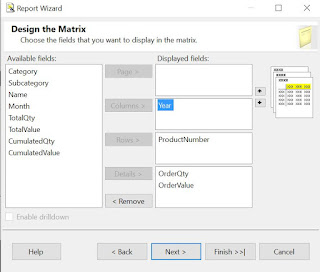
Using the Report Wizard create a new matrix report called "Sales Volume per Product" based on either of the above queries (I considered the second). Within "Design the Matrix" select the attributes as follows:
Design the Matrix

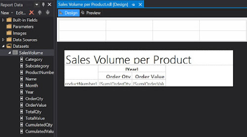
This will create the backbone for our report:

First draft in Design mode

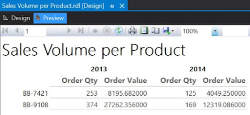
Which is pretty basic, if we consider the output:

First draft in Preview mode

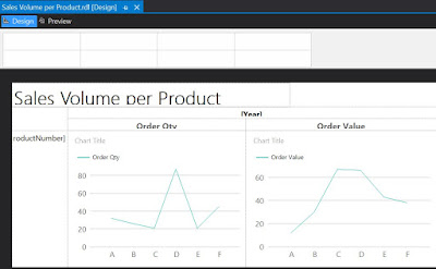
Now, returning in Design mode, right click on the "Sum of OrderQty" cell and from the floating menu select Insert/Chart, while from the list of available charts select Line. Do the same for "Sum of OrderValue". And here's the result:

Second draft in Design mode

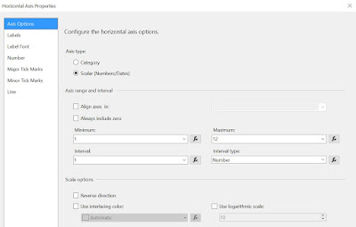
As only one series will be displayed, select the Chart Title and delete the respective label. Delete the Series label as well. When running the report you'll observe that the horizontal axis values are not really appealing. To dix this right click on the respective area and from the floating menu select Horizontal Axis Properties. Within Axis Options section change the Axis type as 'Scalar', enter '1' as Minimum, '12' as Maximum, '1' as Interval and 'Number' as Interval type:

Horizontal Axis Properties

In the same window, within the Labels section select 'Enable auto-fit' and uncheck the "Labels can be offset", respectively the "Labels can be rotated" checkboxes. 

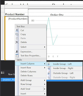
To include the Category, Subcategory and eventually the Product Name, select the Product Number cell, right click on it, and from the floating menu select Insert Column/Inside Group - Left, then select from the Category as attribute:

Inserting a column within the group

Repeat the process to add the Subcategory. Eventually you can add also the Product Name, though for it you'll have to select "Inside Group - Right". 

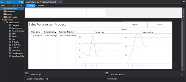
To improve the design, you can add a Page Header and move the report's title into it add a timestamp, respectively a page count textbox, resize the boxes to fit the columns. You can also align the column header values to the center, change the font to 10pt, etc.

Third draft in Design mode

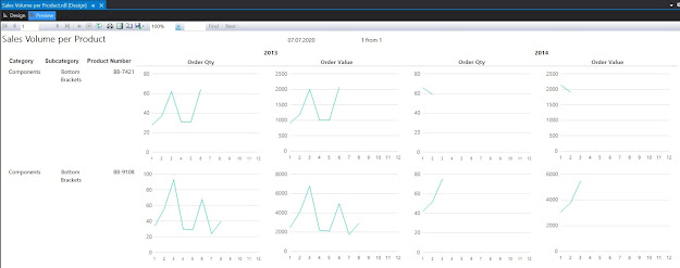
Here's the report in preview mode:

Third draft in Preview mode

One can use the report the way it is, or add the Category and Subcategory as parameters. Similarly, one can use the cumulative values as input for the charts. 

Revamping the Report with Sparklines

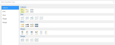
Even if the charts allow displaying the scales, the problem with them is that they are too big, which makes it difficult to compare the data across records. One can correct this by using the other types of graphics available in reports, e.g. sparklines. For this make a copy of the report already built, and within the Detail cells select a Sparkine Column instead of a chart:

Sparkline types


In comparison with Lines, Column-based representations allow to see how many data points are represented. Because spartklines are more compact as graphic forms, you can resize the cells as follows:

Fourth draft in Design mode

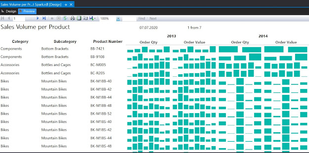
And here's the report in preview mode (the constraints from the source query were removed):

Fourth draft in Preview mode

As can be seen one can easily identify the trends however the volume scale was lost, being impossible to compare which of the Products sold better. One can bring the Total Quantity and Value as display information and sort the dataset from the highest to lowest value. One can even select a top x, to reduce the focus only to the most sold Products.

If the prices remained relatively constant over time, there's actually almost no difference between the graphic displays for Order Quantity, respectively for Order Value. Therefore one can remove one of them (e.g. Order Quantity). Being more compact, sparkline-based representations allow to better use the space, therefore you can add more fields into the report. 

Happy coding!

Previous Post <<||>> Next Post
06 July 2020

🪄SSRS (& Paginated Reports): First Steps (Part IV: Matrix Report Display)

Introduction

SQL Server Reporting Services (SSRS) allows grouping data into a matrix format based on one or more groups. By using the Report Wizard one can simplify considerably the volume of work.

The considered example is based on the AdventureWorks2014 database and considers Product's Inventory as base for building the report. 

Preparing the Data

Usually it's useful to incorporate the logic for a report in one or more views, allowing thus to reuse the views in multiple reports. For the current report is needed to create two views, one for the Products, respectively Production.vProductInventory for the inventory. 

-- dropping the vProducts view (cleaning after)
--DROP VIEW IF EXISTS [Production].[vProducts]

-- creating the vProducts view
CREATE VIEW [Production].[vProducts]
AS 
SELECT p.[ProductID] 
, p.ProductNumber
, p.[Name] 
, IsNull(p.Size, '') + IsNull(' ' + p.SizeUnitMeasureCode, '') Size
, p.Color
, P.Style
, p.ProductModelID
, pm.[Name] AS [ProductModel] 
, p.StandardCost 
, P.ListPrice
, P.SafetyStockLevel
, P.ReorderPoint
, p.SellStartDate 
, p.SellEndDate
, p.ProductSubcategoryID
, PPS.Name Subcategory
, PPS.ProductCategoryID
, PPC.Name Category
, P.MakeFlag
, P.FinishedGoodsFlag
FROM [Production].[Product] p 
     LEFT JOIN [Production].[ProductModel] pm 
       ON p.[ProductModelID] = pm.[ProductModelID] 
	 LEFT JOIN Production.ProductSubcategory PPS
	   ON P.ProductSubcategoryID = PPS.ProductSubcategoryID 
	      LEFT JOIN Production.ProductCategory PPC
		    ON PPS.ProductCategoryID = PPC.ProductCategoryID 
GO

-- reviewing the data 
SELECT *
FROM [Production].[vProducts]

-- checking the view for internal data consistency
SELECT count(*)
FROM [Production].[Product] p 
     LEFT JOIN [Production].[ProductModel] pm 
       ON p.[ProductModelID] = pm.[ProductModelID] 
	 LEFT JOIN Production.ProductSubcategory PPS
	   ON P.ProductSubcategoryID = PPS.ProductSubcategoryID 
	      LEFT JOIN Production.ProductCategory PPC
		    ON PPS.ProductCategoryID = PPC.ProductCategoryID 


-- dropping the vProductInventory view (cleaning after)
--DROP VIEW IF EXISTS Production.vProductInventory

-- creating the view 
CREATE VIEW Production.vProductInventory
AS
SELECT PPI.ProductId 
, PPD.ProductNumber
, PPD.Name ProductName 
, PPD.ProductModel
, PPD.Size
, PPD.Category
, PPD.Subcategory
, PPD.Style
, PPD.StandardCost
, PPD.ListPrice 
, PPD.StandardCost * PPI.Quantity InventoryValue 
, PPD.ListPrice * PPI.Quantity SalesValue
, PPD.MakeFlag
, PPI.Locationid 
, PPL.Name Location 
, PPI.Shelf 
, PPI.Bin 
, PPI.Quantity 
FROM [Production].[ProductInventory] PPI
     JOIN [Production].[vProducts] PPD
	   ON PPI.ProductID = PPD.ProductID
	 JOIN [Production].[Location] PPL
	   ON PPI.LocationID = PPL.LocationID

-- reviewing the data
SELECT *
FROM Production.vProductInventory

-- checking the view for internal data consistency
SELECT count(*)
FROM [Production].[ProductInventory] PPI
     JOIN [Production].[vProducts] PPD
	   ON PPI.ProductID = PPD.ProductID
	 JOIN [Production].[Location] PPL
	   ON PPI.LocationID = PPL.LocationID

Note:
It's important to check the internal consistency of the views or queries used, on whether the logic removes or duplicates data. For this one can run the query for the uppermost table, and add repeatedly one more join for each run to see whether the number of records remains the same. One can shortcut the validation by checking only the number of records from the base table and for the whole query, and only if there are differences use the previously mentioned approach. (This is how I observed that the Production.vProductDetails view is not usable, because it considers only the Products having a valid Model.)

Creating the Report 

We can now use  the Production.vProductInventory view to create the Product Inventory by Location report based on the following query:

-- Product Inventory by Location
SELECT PPI.Category
, PPI.Subcategory
, PPI.ProductNumber
, PPI.ProductName 
, PPI.ProductModel
, PPI.Size
, PPI.Style
, PPI.StandardCost
, PPI.ListPrice
, PPI.Location 
, PPI.Quantity 
, PPI.InventoryValue 
, PPI.SalesValue 
FROM Production.vProductInventory PPI
ORDER BY PPI.Category
, PPI.Subcategory
, PPI.ProductNumber

Note:
The attributes can be provided in the order in which they should be displayed in the report, reducing thus the overhead in the further steps. 

Using the Reporting Wizard via the Add New Report select in the first step the data source, while in the next step provide the above query:

Design the Query

In the next step select the "Matrix" Report Type:

Select the Report Type

Within the "Design the Matrix" section assign the fields as follows (all the fields except the ones considered as Columns and Details will be considered as Rows):

Design the Matrix

Into the last step give the report a meaningful name (e.g. Product Inventory by Location):

Completing the Wizard

In theory the report is ready to run, however before doing that change the formatting by aligning the headers to the center and eventually change their size from 11 to 10 pixels, respectively rename the dataset (e.g. Inventory). To obtain the same information about the grouping as below change into the "Advanced Mode".

Design View

And here's the output (I had to scroll through the pages to find meaningful values, therefore part of the Details header is not shown):

Preview

Restructuring the Grouping

As can be seen into the Design Mode, the wizard created a grouping for each attribute provider into the Details (see matrix1_Category, matrix1_Subcategory, etc.). Therefore, the values will not be repeated for each row, which is typically desirable for visualizations but not when exporting the data to Excel for further processing. I prefer the latter version, therefore to obtain this behavior one can go on and delete all the grouping via "Delete group only" except the matrix1_Category:

Deleting the groups

This action deleted unfortunately all the Detailed headers except Category. To bring them back into the grouping double click on the and add each field into the Group expressions as below:

Group Properties

As final change before running the report one can add header names for the Detail attributes. After these changes reports' design looks as follows:

Report Design with one grouping

And here's the final report with the values repeating for each row:

Preview Report without formatting

Note:
To avoid removing the groupings, I prefer to add only one Detail field into the query, typically the field which will make the row unique into the output (e.g. Product Number) and add the further fields (actually replace the below query with the one above) after the Wizard created the report. One still needs to add the columns manually into the report. In the end the effort is similar. 

-- Product Inventory by Location
SELECT PPI.ProductNumber
, PPI.Location 
, PPI.Quantity 
, PPI.InventoryValue 
, PPI.SalesValue 
FROM Production.vProductInventory PPI
ORDER BY PPI.Category
, PPI.Subcategory
, PPI.ProductNumber

Changing the Design

Report's design can be slightly improved by adding various formatting of the cells or values. One can use similar formatting as the ones consider in the previous post. The only thing difficult to implement will be a ranking function (see Ranking Rows in Reports). After the design changes here's the report:

Final Report

Note:
Of course, together with parameters one can also add totals after each Category or Subcategory to the report if needed, though the latter is more appropriate for design purposes and not for further data consumption. 

Happy coding!

Previous Post <<||>> Next Post
Related Posts Plugin for WordPress, Blogger...

About Me

My photo
Koeln, NRW, Germany
IT Professional with more than 24 years experience in IT in the area of full life-cycle of Web/Desktop/Database Applications Development, Software Engineering, Consultancy, Data Management, Data Quality, Data Migrations, Reporting, ERP implementations & support, Team/Project/IT Management, etc.