🌌🏭KQL Reloaded: First Steps (Part VII: Basic Data Visualizations)

One of the greatest aspects of KQL and its environment is that creating a chart is just one instruction away from the dataset generated in the process. Of course, the data still need to be in an appropriate form to be used as source for a visual, though the effort is minimal. Let's consider the example used in the previous post based ln the ContosoSales data, where the visualization part is everything that comes after "| render":

// visualizations by Country: various charts
NewSales
| where SalesAmount <> 0 and ProductCategoryName == 'TV and Video'
| where DateKey >=date(2023-02-01) and DateKey < datetime(2023-03-01)
| summarize count_customers = count_distinct(CustomerKey) by RegionCountryName
| order by count_customers desc
//| render table
//| render linechart
//| render areachart 

//| render stackedchart
//| render columnchart
| render piechart
    with (xtitle="Country", ytitle="# Customers",
    title="# Customers by Country (pie chart)", legend=hidden)

Output:

# Customers by Country (various charts)

It's enough to use "render" with the chart type without specifying the additional information provided under "with", though the legend can facilitate data's understanding. Unfortunately, the available properties are relatively limited, at least for now. 

Adding one more dimension is quite simple, even if the display may be sometimes confusing as there's no clear delimitation between the entities represented while the legend grows linearly with the number of points. It might be a good idea to use additional charts for the further dimensions in scope. 

// visualizations by Region & Country: various charts
NewSales
| where SalesAmount <> 0 and ProductCategoryName == 'TV and Video'
| where DateKey >=date(2023-02-01) and DateKey < datetime(2023-03-01)
| summarize count_customers = count_distinct(CustomerKey) by ContinentName, RegionCountryName
| order by count_customers desc   
//| render stackedareachart 
//| render linechart 
//| render table 
//| render areachart 
//| render piechart
| render columnchart 
    with (xtitle="Region/Country", ytitle="# Customers",
    title="#Customers by Continent & Country", legend=hidden)

Output:

# Customers by Continent & Country (column chart)

Sometimes, it makes sense to reduce the number of values, recommendation that applies mainly to pie charts:

// visualizations by Zone: pie chart
NewSales
| where SalesAmount <> 0 and ProductCategoryName == 'TV and Video'
| where DateKey >=date(2023-02-01) and DateKey < datetime(2023-03-01)
| summarize count_customers = count_distinct(CustomerKey) by iif(RegionCountryName in ('United States', 'Canada'), RegionCountryName, 'Others')
| render piechart
    with (xtitle="Country", ytitle="Sales volume",
    title="Sales volume by Zone")

Output:

# Customers by Zone (pie chart)

Adding a second set of values (e.g. Total cost) allows to easily create a scatter chart:

// visualization by Occupation: scatter chart
NewSales
| where SalesAmount <> 0 and ProductCategoryName == 'TV and Video'
| where DateKey >=date(2023-02-01) and DateKey < datetime(2023-03-01)
| summarize count_customers = count_distinct(CustomerKey) 
    , TotalCost = sum(TotalCost) by Occupation
| order by count_customers desc
| render scatterchart 
    with (xtitle="# Customers", ytitle="Sales volume",
    title="# Customers vs Sales volume by Occupation", legend=visible )

Output:

# Customers vs Sales volume by Occupation (scatter chart)

The visualizations are pretty simple to build, though one shouldn't expect that one can build a visualization on top of any dataset, at least not without further formatting and eventually code changes. For example, considering the query from the previous post, with a small change one can use the data with a column chart, though this approach might have some limitation (e.g. it doesn't work pie charts):

// calculating percentages from totals: column chart
NewSales
| where SalesAmount <> 0 and ProductCategoryName == 'TV and Video'
//| where DateKey >=date(2023-02-01) and DateKey < datetime(2023-03-01)
| summarize count_customers = count_distinct(CustomerKey)
    , count_customers_US = count_distinctif(CustomerKey, RegionCountryName == 'United States')
    , count_customers_CA = count_distinctif(CustomerKey, RegionCountryName == 'Canada')
    , count_customers_other = count_distinctif(CustomerKey, not(RegionCountryName in ('United States', 'Canada')))
| project Charting = "Country"
    , US = count_customers_US
    , CA = count_customers_CA
    , other = count_customers_other
| render columnchart

    with (xtitle="Region", ytitle="# Customers",
    title="# Customers by Region")

Output:

# Customers by Region (column chart)

There are a few more visuals that will be considered in a next post. Despite the relatively limited set of visuals and properties, the visualizations are useful to get a sense of data's shape, and this with a minimum of changes. Ad-hoc visualizations can help also in data modeling, validating the logic and/or identifying issues in the data when creating the queries, which makes it a great feature. 

Happy coding!

Previous Post <<||>> Next Post

📊Graphical Representation: Graphics We Live By (Part VIII: List of Items in Power BI)

Graphical Representation Series

Introduction

There are situations in which one needs to visualize only the rating, other values, or ranking of a list of items (e.g. shopping cart, survey items) on a scale (e.g. 1 to 100, 1 to 10) for a given dimension (e.g. country, department). Besides tables, in Power BI there are 3 main visuals that can be used for this purpose: the clustered bar chart, the line chart (aka line graph), respectively the slopegraph:

Main Display Methods

Main Display Methods

For a small list of items and dimension values probably the best choice would be to use a clustered bar chart (see A). If the chart is big enough, one can display also the values as above. However, the more items in the list, respectively values in the dimension, the more space is needed. One can maybe focus then only on a subset of items from the list (e.g. by grouping several items under a category), respectively choose which dimension values to consider. Another important downside of this method is that one needs to remember the color encodings. 

This downside applies also to the next method - the use of a line chart (see B) with categorical data, however applying labels to each line simplifies its navigation and decoding. With line charts the audience can directly see the order of the items, the local and general trends. Moreover, a line chart can better scale with the number of items and dimension values.

The third option (see C), the slopegraph, looks like a line chart though it focuses only on two dimension values (points) and categorizes the line as "down" (downward slope), "neutral" (no change) and "up" (upward slope). For this purpose, one can use parameters fields with measures. Unfortunately, the slopegraph implementation is pretty basic and the labels overlap which makes the graph more difficult to read. Probably, with the new set of changes planned by Microsoft, the use of conditional formatting of lines would allow to implement slope graphs with line charts, creating thus a mix between (B) and (C).

This is one of the cases in which the Y-axis (see B and C) could be broken and start with the meaningful values. 

Table Based Displays

Especially when combined with color encodings (see C & G) to create heatmap-like displays or sparklines (see E), tables can provide an alternative navigation of the same data. The color encodings allow to identify the areas of focus (low, average, or high values), while the sparklines allow to show inline the trends. Ideally, it should be possible to combine the two displays.  

Table Displays and the Aster Plot

One can vary the use of tables. For example, one can display only the deviations from one of the data series (see F), where the values for the other countries are based on AUS. In (G), with the help of visual calculations one can also display values' ranking. 

Pie Charts

Pie charts and their variations appear nowadays almost everywhere. The Aster plot is a variation of the pie charts in which the values are encoded in the height of the pieces. This method was considered because the data used above were encoded in 4 similar plots. Unfortunately, the settings available in Power BI are quite basic - it's not possible to use gradient colors or link the labels as below:

Source Data as Aster Plots

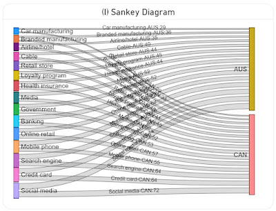
Sankey Diagram

A Sankey diagram is a data visualization method that emphasizes the flow or change from one state (the source) to another (the destination). In theory it could be used to map the items to the dimensions and encode the values in the width of the lines (see I). Unfortunately, the diagram becomes challenging to read because all the lines and most of the labels intersect. Probably this could be solved with more flexible formatting and a rework of the algorithm used for the display of the labels (e.g. align the labels for AUS to the left, while the ones for CAN to the right).

Sankey Diagram

Data Preparation

A variation of the above image with the Aster Plots which contains only the plots was used in ChatGPT to generate the basis data as a table via the following prompts:

• retrieve the labels from the four charts by country and value in a table
• consolidate the values in a matrix table by label country and value

The first step generated 4 tables, which were consolidated in a matrix table in the second step. Frankly, the data generated in the first step should have been enough because using the matrix table required an additional step in DAX.

Here is the data imported in Power BI as the Industries query:

let
    Source = #table({"Label","Australia","Canada","U.S.","Japan"}
, {
 {"Credit card","67","64","66","68"}
, {"Online retail","55","57","48","53"}
, {"Banking","58","53","57","48"}
, {"Mobile phone","62","55","44","48"}
, {"Social media","74","72","62","47"}
, {"Search engine","66","64","56","42"}
, {"Government","52","52","58","39"}
, {"Health insurance","44","48","50","36"}
, {"Media","52","50","39","23"}
, {"Retail store","44","40","33","23"}
, {"Car manufacturing","29","29","26","20"}
, {"Airline/hotel","35","37","29","16"}
, {"Branded manufacturing","36","33","25","16"}
, {"Loyalty program","45","41","32","12"}
, {"Cable","40","39","29","9"}
}
),
    #"Changed Types" = Table.TransformColumnTypes(Source,{{"Australia", Int64.Type}, {"Canada", Int64.Type}, {"U.S.", Number.Type}, {"Japan", Number.Type}})
in
    #"Changed Types"

Transforming (unpivoting) the matrix to a table with the values by country:

IndustriesT = UNION (
    SUMMARIZECOLUMNS(
     Industries[Label]
     , Industries[Australia]
     , "Country", "Australia"
    )
    , SUMMARIZECOLUMNS(
     Industries[Label]
     , Industries[Canada]
     , "Country", "Canada"
    )
    , SUMMARIZECOLUMNS(
     Industries[Label]
     , Industries[U.S.]
     , "Country", "U.S."
    )
    ,  SUMMARIZECOLUMNS(
     Industries[Label]
     , Industries[Japan]
     , "Country", "Japan"
    )
)

Notes:

The slopechart from MAQ Software requires several R language libraries to be installed (see how to install the R language and optionally the RStudio). Run the following scripts, then reopen Power BI Desktop and enable running visual's scripts.

install.packages("XML")
install.packages("htmlwidgets")
install.packages("ggplot2")
install.packages("plotly")

Happy (de)coding!

Previous Post <<||>> Next Post