🌌🏭KQL Reloaded: First Steps (Part VII: Basic Data Visualizations)

One of the greatest aspects of KQL and its environment is that creating a chart is just one instruction away from the dataset generated in the process. Of course, the data still need to be in an appropriate form to be used as source for a visual, though the effort is minimal. Let's consider the example used in the previous post based ln the ContosoSales data, where the visualization part is everything that comes after "| render":

// visualizations by Country: various charts
NewSales
| where SalesAmount <> 0 and ProductCategoryName == 'TV and Video'
| where DateKey >=date(2023-02-01) and DateKey < datetime(2023-03-01)
| summarize count_customers = count_distinct(CustomerKey) by RegionCountryName
| order by count_customers desc
//| render table
//| render linechart
//| render areachart 

//| render stackedchart
//| render columnchart
| render piechart
    with (xtitle="Country", ytitle="# Customers",
    title="# Customers by Country (pie chart)", legend=hidden)

Output:

# Customers by Country (various charts)

It's enough to use "render" with the chart type without specifying the additional information provided under "with", though the legend can facilitate data's understanding. Unfortunately, the available properties are relatively limited, at least for now. 

Adding one more dimension is quite simple, even if the display may be sometimes confusing as there's no clear delimitation between the entities represented while the legend grows linearly with the number of points. It might be a good idea to use additional charts for the further dimensions in scope. 

// visualizations by Region & Country: various charts
NewSales
| where SalesAmount <> 0 and ProductCategoryName == 'TV and Video'
| where DateKey >=date(2023-02-01) and DateKey < datetime(2023-03-01)
| summarize count_customers = count_distinct(CustomerKey) by ContinentName, RegionCountryName
| order by count_customers desc   
//| render stackedareachart 
//| render linechart 
//| render table 
//| render areachart 
//| render piechart
| render columnchart 
    with (xtitle="Region/Country", ytitle="# Customers",
    title="#Customers by Continent & Country", legend=hidden)

Output:

# Customers by Continent & Country (column chart)

Sometimes, it makes sense to reduce the number of values, recommendation that applies mainly to pie charts:

// visualizations by Zone: pie chart
NewSales
| where SalesAmount <> 0 and ProductCategoryName == 'TV and Video'
| where DateKey >=date(2023-02-01) and DateKey < datetime(2023-03-01)
| summarize count_customers = count_distinct(CustomerKey) by iif(RegionCountryName in ('United States', 'Canada'), RegionCountryName, 'Others')
| render piechart
    with (xtitle="Country", ytitle="Sales volume",
    title="Sales volume by Zone")

Output:

# Customers by Zone (pie chart)

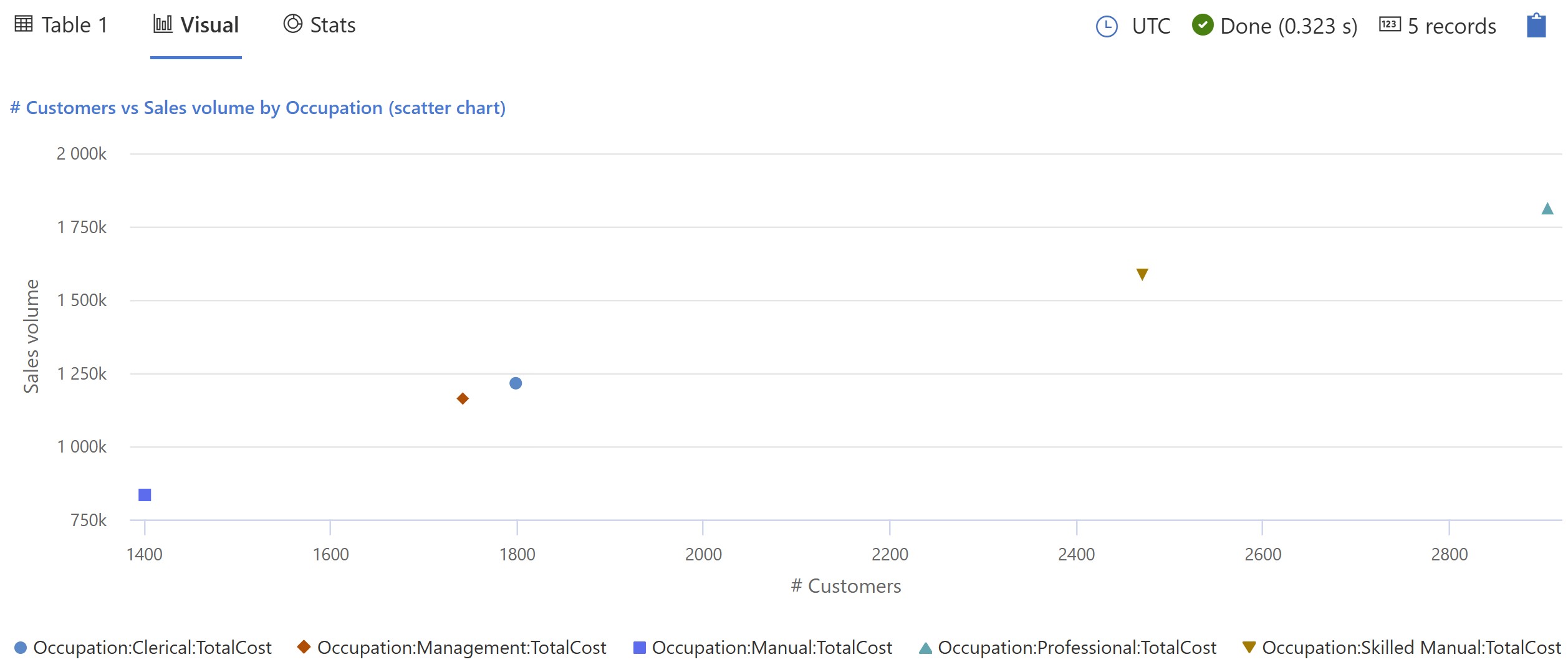
Adding a second set of values (e.g. Total cost) allows to easily create a scatter chart:

// visualization by Occupation: scatter chart
NewSales
| where SalesAmount <> 0 and ProductCategoryName == 'TV and Video'
| where DateKey >=date(2023-02-01) and DateKey < datetime(2023-03-01)
| summarize count_customers = count_distinct(CustomerKey) 
    , TotalCost = sum(TotalCost) by Occupation
| order by count_customers desc
| render scatterchart 
    with (xtitle="# Customers", ytitle="Sales volume",
    title="# Customers vs Sales volume by Occupation", legend=visible )

Output:

# Customers vs Sales volume by Occupation (scatter chart)

The visualizations are pretty simple to build, though one shouldn't expect that one can build a visualization on top of any dataset, at least not without further formatting and eventually code changes. For example, considering the query from the previous post, with a small change one can use the data with a column chart, though this approach might have some limitation (e.g. it doesn't work pie charts):

// calculating percentages from totals: column chart
NewSales
| where SalesAmount <> 0 and ProductCategoryName == 'TV and Video'
//| where DateKey >=date(2023-02-01) and DateKey < datetime(2023-03-01)
| summarize count_customers = count_distinct(CustomerKey)
    , count_customers_US = count_distinctif(CustomerKey, RegionCountryName == 'United States')
    , count_customers_CA = count_distinctif(CustomerKey, RegionCountryName == 'Canada')
    , count_customers_other = count_distinctif(CustomerKey, not(RegionCountryName in ('United States', 'Canada')))
| project Charting = "Country"
    , US = count_customers_US
    , CA = count_customers_CA
    , other = count_customers_other
| render columnchart

    with (xtitle="Region", ytitle="# Customers",
    title="# Customers by Region")

Output:

# Customers by Region (column chart)

There are a few more visuals that will be considered in a next post. Despite the relatively limited set of visuals and properties, the visualizations are useful to get a sense of data's shape, and this with a minimum of changes. Ad-hoc visualizations can help also in data modeling, validating the logic and/or identifying issues in the data when creating the queries, which makes it a great feature. 

Happy coding!

Previous Post <<||>> Next Post

🌌🏭KQL Reloaded: First Steps (Part VI: Actual vs. Estimated Count)

More examples are available nowadays for developers, at least compared with 10-20 years ago when besides the scarce documentation, the blogs and source code from books were the only ways to find how a function or a piece of standard functionality works. Copying code without understanding it may lead to unexpected results, with all the consequences resulting from this. 

A recent example in this direction in KQL are the dcount and dcountif functions, which according to the documentation calculates an estimate of the number of distinct values that are taken by a scalar expression in the summary group. An estimate is not the actual number of records, trading performance for accuracy. The best example are the following pieces of code:

// counting records 
NewSales
| summarize record_count = count() // values availanle 
    , aprox_distinct_count = dcount(CustomerKey) // estimated disting values
    , distinct_count = count_distinct(CustomerKey) // actual number of records
    , aprox_distict_count_by_value  = dcountif(CustomerKey, SalesAmount <> 0) //estimated count of records with not null amounts
    , distict_count_by_value  = count_distinctif(CustomerKey, SalesAmount <> 0) // count of records with not null amounts
    , aprox_distict_count_by_value2  = dcountif(CustomerKey, SalesAmount == 0) //estimated count of records with null amounts
    , distict_count_by_value2  = count_distinctif(CustomerKey, SalesAmount == 0) // count of records with not amounts
| extend error_aprox_distinct_count = distinct_count - aprox_distinct_count
    , error_aprox_distict_count_by_value = distict_count_by_value - aprox_distict_count_by_value

Output:

record_count	aprox_distinct_count	distinct_count	aprox_distict_count_by_value	distict_count_by_value	aprox_distict_count_by_value2	distict_count_by_value2
2832193	18497	18484	18497	18484	10251	10219
error_aprox_distinct_count		error_aprox_distict_count_by_value
-13		-13

It's interesting that the same difference is observable also when a narrower time interval is chosen (e.g. 1 month). When using estimate it's important to understand also how big is the error between the actual value and the estimate, and that's the purpose of the last two lines added to the query. In many scenarios the difference might be neglectable until is not. 

One can wonder whether the two functions are deterministic, in other words whether they return the same results if given the same input values. It would be also useful to understand what's the performance of the two estimative functions especially when further constraints are applied.

Moreover, the functions accept a third parameter which allows control over the trade between speed and accuracy (see provided table).

// counting records 
NewSales
| summarize record_count = count() // values availanle 
    , distinct_count = count_distinct(CustomerKey) // actual number of records
    , aprox_distinct_count = dcount(CustomerKey) // estimated disting values (default)
    , aprox_distinct_count0 = dcount(CustomerKey, 0) // 0-based accuracy
    , aprox_distinct_count1 = dcount(CustomerKey, 1) // 1-based accuracy (default)
    , aprox_distinct_count2 = dcount(CustomerKey, 2) // 2-based accuracy
    , aprox_distinct_count3 = dcount(CustomerKey, 3) // 3-based accuracy
    , aprox_distinct_count4 = dcount(CustomerKey, 4) // 4-based accuracy

Output:

record_count	distinct_count	aprox_distinct_count	aprox_distinct_count0	aprox_distinct_count1	aprox_distinct_count2	aprox_distinct_count3	aprox_distinct_count4
2832193	18484	18497	18793	18497	18500	18470	18487

It will be interesting to see which one of these parameters are used in practice. The problems usually start when different approximation parameters are used alternatively with no previous agreement. How could one argument in the favor of one parameter over the others? 

A natural question: how big will be the error introduced by each parameter? Usually, when approximating values, one needs to specify also the expected error somehow. The documentation provide some guiding value, though are these values enough? Do similar estimate functions make sense also for the other aggregate functions?

In exchange, the count_distinct and count_distinctif seem to be still in preview, with all the consequences derived from this. They are supposed to be more resource-intensive than the estimative counterparts. Conversely, the values returned can be still rounded in dashboards up to the meaningful unit (e.g. thousands), and this usually depends on the context. The question whether the values can be rounded can be put also in the context and the estimative counterparts. It would be interesting to check how far away are the rounded values from each other in the context of the two sets of functions.

In practice, counting is useful for calculating percentages (e.g. how many customers come from a certain zone compared to the total), which are more useful and easier to grasp than big numbers: 

// calculating percentages from totals
NewSales
| where SalesAmount <> 0 and ProductCategoryName == 'TV and Video'
| where DateKey >=date(2023-02-01) and DateKey < datetime(2023-03-01)
| summarize count_customers = count_distinct(CustomerKey)
    , count_customers_US = count_distinctif(CustomerKey, RegionCountryName == 'United States')
    , count_customers_CA = count_distinctif(CustomerKey, RegionCountryName == 'Canada')
    , count_customers_other = count_distinctif(CustomerKey, not(RegionCountryName in ('United States', 'Canada')))
| extend percent_customers_US = iif(count_customers<>0, round(100.00 * count_customers_US/count_customers, 2), 0.00)
    , percent_customers_CA = iif(count_customers<>0, round(100.00 * count_customers_CA/count_customers, 2), 0.00)
    , percent_customers_other = iif(count_customers<>0, round(100.00 * count_customers_other/count_customers,2), 0.00)

Output:

count_customers	count_customers_US	count_customers_CA	count_customers_other	percent_customers_US	percent_customers_CA	percent_customers_other
10317	3912	789	5616	37.92	7.65	54.43

Note:
When showing percentages it's important to provide also the "context", the actual count or amount. This allows to understand the scale associated with the percentages. 

Happy coding!

Previous Post <<||>> Next Post

Resources:
[R1] Arcane Code (2022) Fun With KQL – DCount, by R C Cain [link]

[R2] M Morowczynsk et al (2024) "The Definitive Guide to KQL" [sample]
[R3] M Zorich (2022) Too much noise in your data? Summarize it! [link]

💎🏭SQL Reloaded: The WINDOW Clause in SQL Server 2022 (Part I: Simple Aggregations)

Between the many new features introduced in SQL Server 2022, Microsoft brings the WINDOW clause for defining the partitioning and ordering of a dataset which uses window functions. But before unveiling the change, let's take a walk down the memory lane.

In the early ages of SQL Server, many of descriptive statistics techniques were resuming in using the averages over a dataset that contained more or less complex logic. For example, to get the total and average of sales per Month, the query based on AdventureWorks database would look something like:

-- aggregated sales orders - detailed (SQL Server 2000+)
SELECT SOL.ProductID
, Year(SOH.OrderDate) [Year]
, Month(SOH.OrderDate) [Month]
, SUM(SOL.OrderQty) TotalQty
, AVG(SOL.OrderQty) AverageQty
FROM Sales.SalesOrderDetail SOL
     JOIN Sales.SalesOrderHeader SOH
	   ON SOL.SalesOrderID = SOH.SalesOrderID
WHERE SOL.ProductId IN (745)
  AND Year(SOH.OrderDate) = 2012
  AND Month(SOH.OrderDate) BETWEEN 1 AND 3
GROUP BY SOL.ProductID
, Year(SOH.OrderDate) 
, Month(SOH.OrderDate)

When possible, the base logic was encapsulated within a view, hiding query's complexity from the users, allowing also reuse and better maintenance, just to mention a few of the benefits of this approach:

-- encapsulating the logic into a view (SQL Server 2000+)
CREATE OR ALTER VIEW Sales.vSalesOrders
AS
-- sales orders details
SELECT SOL.SalesOrderID
, SOL.ProductID
, Cast(SOH.OrderDate as Date) OrderDate
, Year(SOH.OrderDate) [Year]
, Month(SOH.OrderDate) [Month]
, Cast(SOL.OrderQty as decimal(18,2)) OrderQty
-- many more columns 
FROM Sales.SalesOrderDetail SOL
     JOIN Sales.SalesOrderHeader SOH
	   ON SOL.SalesOrderID = SOH.SalesOrderID
/* -- some constraints can be brought directly into the view
WHERE SOL.ProductID IN (745)
  AND Year(SOH.OrderDate) = 2012
  AND Month(SOH.OrderDate) BETWEEN 1 AND 3
*/

The above query now becomes:

 

-- aggregated sales orders - simplified (SQL Server 2000+)
SELECT SOL.ProductID
, SOL.[Year]
, SOL.[Month]
, SUM(SOL.OrderQty) TotalQty
, AVG(SOL.OrderQty) AverageQty
FROM Sales.vSalesOrders SOL
WHERE SOL.ProductID IN (745)
  AND SOL.[Year] = 2012
  AND SOL.[Month] BETWEEN 1 AND 3
GROUP BY SOL.ProductID
, SOL.[Year]
, SOL.[Month]

In many cases, performing this kind of aggregations was all the users wanted. However, quite often it's useful to look and the individual sales and consider them as part of the broader picture. For example, it would be interesting to know, what's the percentage of an individual value from the total (see OrderQtyPct) or any similar aggregate information. In SQL Server 2000 addressing such requirements would involve a join between the same view - one query with the detailed records, while the other contains the aggregated data:

-- sales orders from the totals (SQL Server 2000+)
SELECT SOL.*
, ASO.TotalQty
, Cast(CASE WHEN ASO.TotalQty <> 0 THEN 100*SOL.OrderQty/ASO.TotalQty ELSE 0 END as decimal(18,2)) OrderQtyPct
, ASO.AverageQty
FROM Sales.vSalesOrders SOL
     JOIN ( -- aggregated sales orders
		SELECT SOL.ProductID
		, SOL.[Year]
		, SOL.[Month]
		, SUM(SOL.OrderQty) TotalQty
		, AVG(SOL.OrderQty) AverageQty
		FROM Sales.vSalesOrders SOL
		WHERE SOL.ProductID IN (745)
		  AND SOL.[Year] = 2012
		  AND SOL.[Month] BETWEEN 1 AND 3
		GROUP BY SOL.ProductId
		, SOL.[Year]
		, SOL.[Month]
	) ASO
	ON SOL.ProductID = ASO.ProductID 
   AND SOL.[Year] = ASO.[Year]
   AND SOL.[Month] = ASO.[Month]
ORDER BY SOL.ProductID
, SOL.OrderDate

Now, just imagine that you can't create a view and having to duplicate the logic each time the view is used! Aggregating the data at different levels would require similar joins to the same view or piece of logic. 

Fortunately, SQL Server 2005 came with two long-awaited features, common table expressions (CTEs) and window functions, which made a big difference. First, CTEs allowed defining inline views that can be referenced multiple times. Secondly, the window functions allowed aggregations within a partition.

 

-- sales orders with CTE SQL Server 2005+ query 
WITH CTE
AS (--sales orders in scope
SELECT SOL.SalesOrderID 
, SOL.ProductID
, Cast(SOH.OrderDate as Date) OrderDate
, Year(SOH.OrderDate) [Year]
, Month(SOH.OrderDate) [Month]
, SOL.OrderQty
FROM Sales.SalesOrderDetail SOL
     JOIN Sales.SalesOrderHeader SOH
	   ON SOL.SalesOrderID = SOH.SalesOrderID
WHERE SOL.ProductID IN (745)
  AND Year(SOH.OrderDate) = 2012
  AND Month(SOH.OrderDate) BETWEEN 1 AND 3
)
SELECT SOL.SalesOrderID 
, SOL.ProductID
, SOL.OrderDate
, SOL.[Year]
, SOL.[Month]
, SOL.OrderQty
, SUM(SOL.OrderQty) OVER(PARTITION BY SOL.[Year], SOL.[Month]) TotalQty
, AVG(SOL.OrderQty)  OVER(PARTITION BY SOL.[Year], SOL.[Month]) AverageQty
FROM CTE SOL
WHERE SOL.ProductID IN (745)
  AND SOL.[Year] = 2012
  AND SOL.[Month] BETWEEN 1 AND 3

This kind of structuring the queries allows to separate the base logic for better maintainability, readability and fast prototyping. Once the logic from CTE becomes stable, it can be moved within a view, following to replace the CTE reference with view's name in the final query. On the other side, the window functions allow writing more flexible and complex code, even if the statements can become occasionally complex (see OrderQtyPct):

 

-- aggregated sales orders (SQL Server 2005+)
SELECT SOL.SalesOrderID 
, SOL.ProductID
, SOL.OrderDate
, SOL.[Year]
, SOL.[Month]
, SOL.OrderQty
, SUM(SOL.OrderQty) OVER(PARTITION BY SOL.[Year], SOL.[Month]) TotalQty
, AVG(SOL.OrderQty)  OVER(PARTITION BY SOL.[Year], SOL.[Month]) AverageQty
, Cast(CASE WHEN SUM(SOL.OrderQty) OVER(PARTITION BY SOL.[Year], SOL.[Month]) <> 0 THEN 100*SOL.OrderQty/SUM(SOL.OrderQty) OVER(PARTITION BY SOL.[Year], SOL.[Month]) ELSE 0 END as decimal(18,2)) OrderQtyPct
FROM Sales.vSalesOrders SOL
WHERE SOL.ProductID IN (745)
  AND SOL.[Year] = 2012
  AND SOL.[Month] BETWEEN 1 AND 3

Now, SQL Server 2022 allows to further simplify the logic by allowing to define with a name the window at the end of the statement and reference the name in several window functions (see last line of the query):

-- Aggregations per month (SQL Server 2022+)
SELECT SOL.SalesOrderID 
, SOL.ProductID
, SOL.OrderDate
, SOL.[Year]
, SOL.[Month]
, SOL.OrderQty
, SUM(SOL.OrderQty) OVER SalesByMonth AS TotalQty
, AVG(SOL.OrderQty) OVER SalesByMonth AS AverageQty
, Cast(CASE WHEN SUM(SOL.OrderQty) OVER SalesByMonth <> 0 THEN 100*SOL.OrderQty/SUM(SOL.OrderQty) OVER SalesByMonth ELSE 0 END as decimal(18,2)) OrderQtyPct
FROM Sales.vSalesOrders SOL
WHERE SOL.ProductID IN (745)
  AND SOL.[Year] = 2012
  AND SOL.[Month] BETWEEN 1 AND 3
WINDOW SalesByMonth AS (PARTITION BY SOL.[Year], SOL.[Month])

Moreover, several windows can be defined. For example, aggregating the data also per year:

-- Aggregations per month and year (SQL Server 2022+) 
SELECT SOL.SalesOrderID 
, SOL.ProductID
, SOL.OrderDate
, SOL.[Year]
, SOL.[Month]
, SOL.OrderQty
, SUM(SOL.OrderQty) OVER SalesByMonth AS TotalQtyByMonth
, AVG(SOL.OrderQty) OVER SalesByMonth AS AverageQtyByMonth
, Cast(CASE WHEN SUM(SOL.OrderQty) OVER SalesByMonth <> 0 THEN 100*SOL.OrderQty/SUM(SOL.OrderQty) OVER SalesByMonth ELSE 0 END as decimal(18,2)) OrderQtyPctByMonth
, SUM(SOL.OrderQty) OVER SalesByYear AS TotalQtyByYear
, AVG(SOL.OrderQty) OVER SalesByYear AS AverageQtyByYear
, Cast(CASE WHEN SUM(SOL.OrderQty) OVER SalesByYear <> 0 THEN 100*SOL.OrderQty/SUM(SOL.OrderQty) OVER SalesByYear ELSE 0 END as decimal(18,2)) OrderQtyPctByYear
FROM Sales.vSalesOrders SOL
WHERE SOL.ProductID IN (745)
  AND SOL.[Year] = 2012
  AND SOL.[Month] BETWEEN 1 AND 3
WINDOW SalesByMonth AS (PARTITION BY SOL.[Year], SOL.[Month])
, SalesByYear AS  (PARTITION BY SOL.[Year])

Isn't that cool? It will take probably some time to get used in writing and reading this kind of queries, though using descriptive names for the windows should facilitate the process! 

As a side note, even if there's no product function like in Excel, there's a mathematical trick to transform a product into a sum of elements by applying the Exp (exponential) and Log (logarithm) functions (see example).

Notes:
The queries work also in a SQL databases in Microsoft Fabric. Just replace the Sales with SalesLT schema (see post, respectively GitHub repository with the changed code).

Happy coding!

💎🏭SQL Reloaded: Query Patterns in SQL Server (Part IV: Window Functions)

For a long time aggregate functions were the only tool for statistical purposes available for raw SQL scripting. Their limitations become more evident with the introduction of window functions, which allow to apply the aggregates over a defined partition. Besides aggregate window functions, the use of ranking, respectively value window functions, opened the door to a new set of techniques. Here are a few examples based on the tables defined in a previous post.

Ranking windows functions allow ranking a record within the whole dataset or a partition by providing a sorting key:

-- Ranking window functions (RANK, DENSE_RANK, ROW_NUMBER)
SELECT A.CourseId 
, C.CourseName 
, A.StudentId 
, S.StudentName 
, A.StartDate 
, A.EndDate 
, RANK() OVER (ORDER BY A.Mark) [Rank over whole set]
, DENSE_RANK() OVER (ORDER BY A.Mark) [Dense Rank over whole set]
, ROW_NUMBER() OVER (ORDER BY A.Mark) [Row Number over whole set]
--, RANK() OVER (PARTITION BY A.CourseId ORDER BY A.StartDate) [Rank over Course]
--, RANK() OVER (PARTITION BY A.StudentId ORDER BY A.StartDate) [Rank over Student]
--, DENSE_RANK() OVER (PARTITION BY A.CourseId ORDER BY A.StartDate) [Dense Rank over Course]
--, DENSE_RANK() OVER (PARTITION BY A.StudentId ORDER BY A.StartDate) [Dense Rank over Student]
--, ROW_NUMBER() OVER (PARTITION BY A.CourseId ORDER BY A.StartDate) [Dense Rank over Course]
--, ROW_NUMBER() OVER (PARTITION BY A.StudentId ORDER BY A.StartDate) [Dense Rank over Student]
FROM dbo.T_Allocations A
     JOIN dbo.T_Courses C
       ON A.CourseId = C.CourseId 
     JOIN dbo.T_Students S
       ON A.StudentId = S.StudentId 
ORDER BY C.CourseName 
, S.StudentName 

Being able to rank records allows to easier select the last, respectively the first records from a dataset or a given partition:

-- first course 
SELECT *
, A.StartDate 
FROM dbo.T_Students S
     LEFT JOIN (
		SELECT A.CourseId
		, A.StudentId 
		, A.StartDate 
		, RANK() OVER (PARTITION BY A.StudentId ORDER BY A.StartDate) Ranking 
		FROM dbo.T_Allocations A
    ) A
   ON S.StudentId = A.StudentId 
  AND A.Ranking = 1 
ORDER BY S.StudentName

The aggregate window functions function similarly as their simple counterparts, except that they are valid over a partition. If the partition is left out, the functions apply over the whole data set.

-- aggregate window functions 
SELECT A.CourseId 
, C.CourseName 
, A.StudentId 
, S.StudentName 
, A.StartDate 
, A.EndDate 
, SUM(A.Mark) OVER (PARTITION BY A.StudentId) [Sum]
, MAX(A.Mark) OVER (PARTITION BY A.StudentId) [Max]
, MIN(A.Mark) OVER (PARTITION BY A.StudentId) [Min]
, AVG(A.Mark) OVER (PARTITION BY A.StudentId) [Avg]
, COUNT(A.Mark) OVER (PARTITION BY A.StudentId) [Count]
FROM dbo.T_Allocations A
     JOIN dbo.T_Courses C
       ON A.CourseId = C.CourseId 
     JOIN dbo.T_Students S
       ON A.StudentId = S.StudentId 
ORDER BY C.CourseName 
, S.StudentName 

When the ordering attributes are specified, running averages, respectively sums derive:

-- Running averages/sums and ranking via Sum and ORDER BY
SELECT A.StudentId 
, A.CourseId
, A.StartDate
, A.EndDate
, A.Mark 
, AVG(Cast(Mark as decimal(4,2))) OVER (PARTITION BY A.StudentId ORDER BY A.StartDate, A.AllocationId) AvgGrade
, SUM(Mark) OVER (PARTITION BY A.StudentId ORDER BY A.StartDate, A.AllocationId) SumGrade
, RANK() OVER (PARTITION BY A.StudentId ORDER BY A.StartDate, A.AllocationId) Ranking
FROM dbo.T_Allocations A
ORDER BY A.StudentId
, A.StartDate

Running averages were introduced only with SQL Server 2008. Previously, one could still calculate them using common table expressions and a ranking function:

 

-- Running averages/sums and ranking via common table expressions 
WITH CTE AS (
	SELECT A.StudentId 
	, A.CourseId
	, A.StartDate
	, A.EndDate
	, A.Mark 
	, RANK() OVER (PARTITION BY A.StudentId ORDER BY A.StartDate, A.AllocationId) Ranking
	FROM dbo.T_Allocations A
), 
DAT AS (
	SELECT A.StudentId 
	, A.CourseId
	, A.StartDate
	, A.EndDate
	, A.Mark 
	, A.Ranking
	, A.Mark SumMark
	FROM CTE A
	WHERE A.Ranking = 1
	UNION ALL
	SELECT CTE.StudentId 
	, CTE.CourseId
	, CTE.StartDate
	, CTE.EndDate
	, CTE.Mark 
	, CTE.Ranking
	, CTE.Mark + DAT.Mark SumMark 
	FROM CTE
		 JOIN DAT
		   ON CTE.StudentID = DAT.StudentId 
		  AND CTE.Ranking-1 = DAT.Ranking 
) 
SELECT DAT.StudentId 
, DAT.CourseId
, DAT.StartDate
, DAT.EndDate
, DAT.Mark 
, cast(DAT.SumMark/DAT.Ranking as decimal(4,2)) AvgMark
, DAT.SumMark
, DAT.Ranking
FROM DAT
ORDER BY DAT.StudentId
, DAT.StartDate
   

Notes:

The queries work also in SQL databases in Microsoft Fabric.

Happy coding!

Previous Post <<||>> Next Post