
|
|
Graphical Representation Series
|
An exchange rate (XR) is the rate at which one currency will be exchanged for
another currency, and thus XRs are used in everything related to trades,
several processes in Finance relying on them. There are various sources for
the XR like the European Central Bank (ECB) that provide the row data and
various analyses including graphical representations varying in complexity.
Conversely, XRs' processing offers some opportunities for learning techniques
for data visualization.
On ECB there are
monthly, yearly, daily and biannually XRs from EUR to the various currencies which by
triangulation allow to create XRs for any of the currencies involved. If N
currencies are involved for one time unit in the process (e.g. N-1 XRs) , the
triangulation generates NxN values for only one time division, the result
being tedious to navigate. A matrix like the one below facilitates identifying
the value between any of the currencies:
The table needs to be multiplied by 12, the number of months, respectively by
the number of years, and filter allowing to navigate the data as needed. For
many operations is just needed to look use the EX for a given time division.
There are however operations in which is needed to have a deeper understanding
of one or more XR's evolution over time (e.g. GBP to NOK).
Moreover, for some operations is enough to work with two decimals, while for
others one needs to use up to 6 or even more decimals for each XR.
Occasionally, one can compromise and use 3 decimals, which should be enough
for most of the scenarios. Making sense of such numbers is not easy for most
of us, especially when is needed to compare at first sight values across
multiple columns. Summary tables can help:
Statistics like Min. (minimum), Max. (maximum), Max. - Min. (range), Avg.
(average) or even StdDev. (standard deviation) can provide some basis for
further analysis, while sparklines are ideal for showing trends over a time
interval (e.g. months).
Usually, a heatmap helps to some degree to navigate the data, especially when
there's a plot associated with it:
In this case filtering by column in the heatmap allows to see how an XR
changed for the same month over the years, while the trendline allows to
identify the overall tendency (which is sensitive to the number of years
considered). Showing tendencies or patterns for the same month over several
years complements the yearly perspective shown via sparklines.
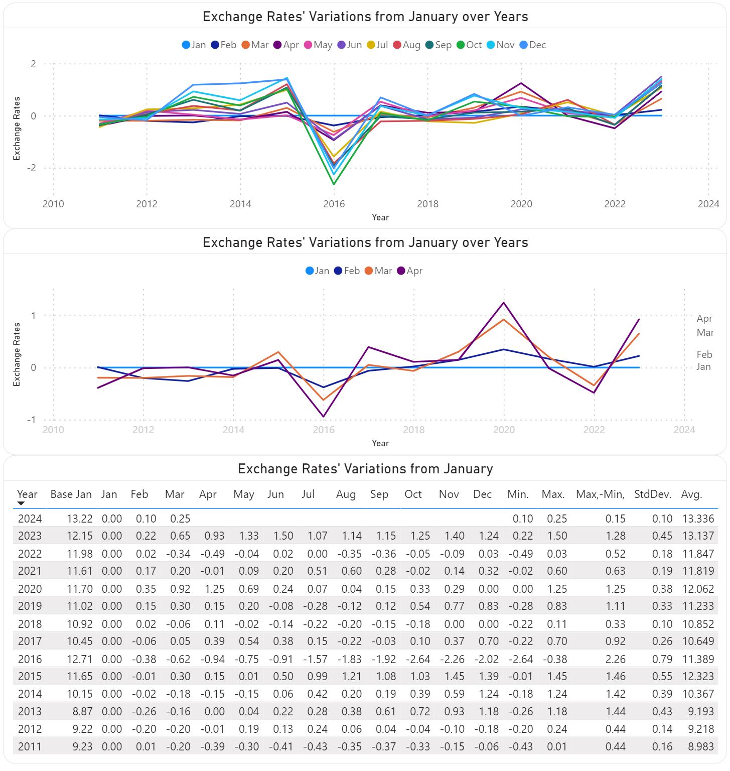
Fortunately, there are techniques to reduce the representational complexity of
such numbers. For example, one can use as basis the XRs for January (see Base
Jan), and represent the other XRs only as differences from the respective XR.
Thus, in the below table for February is shown the XR difference between
February and January (13.32-13.22=0.10). The column for January is zero and
could be omitted, though it can still be useful in further calculations (e.g.
in the calculation of averages) based on the respective data..

This technique works when the variations are relatively small (e.g. the values
vary around 0). The above plots show the respective differences for the whole
year, respectively only for four months. Given a bigger sequence (e.g. 24, 28
months) one can attempt to use the same technique, though there's a point
beyond which it becomes difficult to make sense of the results. One can also
use the year end XR or even the yearly average for the same, though it adds
unnecessary complexity to the calculations when the values for the whole year
aren't available.
Usually, it's recommended to show only 3-5 series in a plot, as one can better
distinguish the trends. However, plotting all series allows to grasp the
overall pattern, if any. Thus, in the first plot is not important to identify
the individual series but to see their tendencies. The two perspectives can be
aggregated into one plot obtained by applying different filtering.
Of course, a similar perspective can be obtained by looking at the whole XRs:
The Max.-Min. and StdDev (standard deviation for population) between the last
and previous tables must match.
Certain operations require comparing the trends of two currencies. The first
plot shows the evolution NOK and SEK in respect to EUR, while the second shows
only the differences between the two XRs:
The first plot will show different values when performed against other
currency (e.g. USD), however the second plot will look similarly, even if the
points deviate slightly:
Another important difference is the one between monthly and yearly XRs,
difference depicted by the below plot:
The value differences between the two XR types can have considerable impact on
reporting. Therefore, one must reflect in analyses the rate type used in the
actual process.
Attempting to project data into the future can require complex techniques,
however, sometimes is enough to highlight a probable area, which depends also
on the confidence interval (e.g. 85%) and the forecast length (e.g. 10
months):
Every perspective into the data tends to provide something new that helps in
sense-making. For some users the first table with flexible filtering (e.g.
time unit, currency type, currency from/to) is enough, while for others
multiple perspectives are needed. When possible, one should allow users
to explore the various perspectives and use the feedback to remove or even add
more perspectives. Including a feedback loop in graphical representation is
important not only for tailoring the visuals to users' needs but also for
managing their expectations, respectively of learning what works and
what doesn't.
Comments:
1) I used GBP to NOK XRs to provide an example
based on triangulation.
2) Some experts advise against using
borders or grid lines. Borders, as the name indicates allow to delimitate
between various areas, while grid lines allow to make comparisons within a
section without needing to sway between broader areas, adding thus precision
to our senses-making. Choosing grey as color for the elements from the
background minimizes the overhead for coping with more information while
allowing to better use the available space.
3) Trend lines are
recommended where the number of points is relatively small and only one series
is involved, though, as always, there are exceptions too.
4) In
heatmaps one can use a gradient between two colors to show the tendencies of
moving toward an extreme or another. One should avoid colors like red or
green.
5) Ideally, a color should be used for only one encoding (e.g. one
color for the same month across all graphics), though the more elements need
to be encoded, the more difficult it becomes to respect this rule. The above
graphics might slightly deviate from this as the purpose is to show a
representation technique.
6) In some graphics the XRs are displayed
only with two decimals because currently the technique used (visual calculations) doesn't support formatting.
7) All the above graphical elements are
based on a Power BI solution. Unfortunately, the tool has its representational
limitations, especially when one wants to add additional information into the
plots.
8) Unfortunately, the daily XR values are not easily
available from the same source. There are special scenarios for which a daily,
hourly or even minute-based analysis is needed.
9) It's a good idea to
validate the results against the similar results available on the web (see the
ECB website).
Previous Post
<<||>>
Next Post


No comments:
Post a Comment