"An integrated, centralized decision support database and the related software programs used to collect, cleanse, transform, and store data from a variety of operational sources to support Business Intelligence. A Data Warehouse may also include dependent data marts." (DAMA International, The DAMA Guide to the Data Management Body of Knowledge 1st Ed., 2009)
"(1) A centralized database for collecting the data from numerous other systems so that they can be made available for management reporting. The database is close to 3rd Normal Form. (2) A system that includes the central database described in 1; plus procedures for extracting, transforming, and loading data from other systems; and one or more data marts that organize subsets of the data for particular reporting purposes." (David C Hay, "Data Model Patterns: A Metadata Map", 2010)
"[A] data warehouse is a collection of data designed to support management in the decision-making process. It is a subject oriented, integrated, time-variant, non-up datable collection of data used in support of management decision-making processes and business intelligence. It contains a wide variety of data that present a coherent picture of business condition at a single point of time. It is a unique kind of database which focuses on business intelligence, external data and time-variant data." (Vijay K Pallaw, "Database Management Systems" 2nd Ed., 2010)
"A data warehouse is a large, enterprise-wide database that acts as a central storage location for data that has been through the Extract, Transform, and Load (ETL) process. A data warehouse often includes historical data as well." (Ken Withee, "Microsoft Business Intelligence For Dummies", 2010)
[Active Data Warehouse (ADW):] "A data warehouse that is generally capable of supporting near-real-time updates, fast response times, and mixed workloads by leveraging well-architected data models, optimized ETL processes, and the use of workload management." (Martin Oberhofer et al, "The Art of Enterprise Information Architecture", 2010)
"A large, often enterprise-wide repository of data used for reporting and analysis. Data warehouses generally collect and manage data from a large number of operational and financial systems across an enterprise." (Janice M Roehl-Anderson, "IT Best Practices for Financial Managers", 2010)
"A subject-oriented, integrated, time-variant, and historical collection of summary and detailed data used to support the decision-making and other reporting and analysis needs that require historical, point-in-time information. Data, once captured within the warehouse, is nonvolatile and relevant to a point in time." (David Lyle & John G Schmidt, "Lean Integration", 2010)
"A specialized type of database that is used to aggregate data from transaction databases for data analysis purposes, such as identifying and examining business trends, to support planning and decision making." (Linda Volonino & Efraim Turban, "Information Technology for Management" 8th Ed, 2011)
[Enterprise Data Warehousing (EDW):] "A data repository of organizational data that is organized, analyzed, and used to enable more informed decision making and planning." (Linda Volonino & Efraim Turban, "Information Technology for Management" 8th Ed, 2011)
[federated data warehouse:] "1.A conceptual Data Warehouse made up of multiple decision support databases, potentially on multiple servers, but presented transparently to Business Intelligence users as a unified schema for query, analysis, and reporting. 2.An Enterprise Data Warehouse fed by extracts from departmental Data Warehouses and/or legacy Data Warehouses prior to their incorporation and/or retirement." (DAMA International, "The DAMA Dictionary of Data Management", 2011)
"The database that stores operations data for long periods of time." (Microsoft, "SQL Server 2012 Glossary", 2012)
"A database used for reporting and analysis." (Craig S Mullins, "Database Administration", 2012)
"A large data store containing the organization’s historical data, which is used primarily for data analysis and data mining. It is the data system of record." (Marcia Kaufman et al, "Big Data For Dummies", 2013)
"A shared repository of data, often used to support the centralized consolidation of information for decision support." (Evan Stubbs, "Delivering Business Analytics: Practical Guidelines for Best Practice", 2013)
"A shared repository of data, often used to support the centralized consolidation of information for decision support." (Evan Stubbs, "Delivering Business Analytics: Practical Guidelines for Best Practice", 2013)
"A store that provides data from the originating source or the operational data stores; it contains historical and derived data. Also known as an information warehouse." (Brenda L Dietrich et al, "Analytics Across the Enterprise", 2014)
"A subject-oriented, integrated, nonvolatile, time-variant collection of data in support of management’s decisions" (Daniel Linstedt & W H Inmon, "Data Architecture: A Primer for the Data Scientist", 2014)
"A large data store containing the organization’s historical data, which is used primarily for data analysis and data mining. It is the data system of record." (Judith S Hurwitz, "Cognitive Computing and Big Data Analytics", 2015)
"A centralized database system which captures data and allows later analysis of the collected data." (Hamid R Arabnia et al, "Application of Big Data for National Security", 2015)
"A secondary database that holds older data for analysis. In some applications, you may want to analyze the data and store modified or aggregated forms in the warehouse instead of keeping every outdated record." (Rod Stephens, "Beginning Software Engineering", 2015)
"Decision-making data base containing the totality of a business’ decision-making data (all subjects)." (Fernando Iafrate, "From Big Data to Smart Data", 2015)
[Enterprise Data Warehouse (EDW):] "A clean data store created to merge and store data from different sources for enterprise data analysis." (David K Pham, "From Business Strategy to Information Technology Roadmap", 2016)
"A granular, time-variant, structured store of historical data in a neutral, nonredundant format for multiple uses. Its purpose is the reuse of data." (Gregory Lampshire et al, "The Data and Analytics Playbook", 2016)
"Electronic storehouses where vast amounts of data are arrayed, integrated, categorised, stored, and sold." (K N Krishnaswamy et al, "Management Research Methodology: Integration of Principles, Methods and Techniques", 2016)
"A repository for storing business-relevant data." (Jonathan Ferrar et al, "The Power of People", 2017)
"A very large database designed to support decision making in organizations. It is usually batch updated and structured for rapid online queries and managerial summaries. A data warehouse is a subject-oriented, integrated, time-variant, nonvolatile collection of data." (Daniel J Power & Ciara Heavin, "Decision Support, Analytics, and Business Intelligence" 3rd Ed., 2017)
"A data warehouse is a repository for all the data that an enterprise collects from internal and external sources." (Amar Sahay, "Business Analytics" Vol. I, 2018)
"A data warehouse is a repository of enterprise data used for reporting and analysis." (Michelle Gutzait et al, "Hands-On Data Warehousing with Azure Data Factory", 2018)
"A subject-oriented collection of data that is used to support strategic decision making. The warehouse is the central point of data integration for business intelligence. It is the source of data for data marts within an enterprise and delivers a common view of enterprise data." (Sybase, "Open Server Server-Library/C Reference Manual", 2019)
[Enterprise Data Warehouse (EDW):] "system used for analysis and reporting that consists of central repositories of integrated data from a wide spectrum of different sources." (Francesco Corea, "An Introduction to Data: Everything You Need to Know About AI, Big Data and Data Science", 2019)
"A data warehouse is a subject-oriented, integrated, time-variant, and nonvolatile collection of data that supports management’s decision-making process." (Piethein Strengholt, "Data Management at Scale", 2020)
"A cloud data warehouse is an enterprise data warehouse offered as a managed service (PaaS) on public clouds with optimized integrations for data ingestion, analytics processing, and BI analytics." (Rukmani Gopalan, "The Cloud Data Lake: A Guide to Building Robust Cloud Data Architecture", 2022)
"A data warehouse is a central storage for all data that an enterprise’s various business systems collect." (Logi Analytics) [source]
"A data warehouse is a data management solution to store large quantities of historical business data, performing queries to support various business intelligence and analytics use cases." (Qlik) [source]
"A data warehouse is a database designed to enable business intelligence activities: it exists to help users understand and enhance their organization's performance. It is designed for query and analysis rather than for transaction processing, and usually contains historical data derived from transaction data, but can include data from other sources. Data warehouses separate analysis workload from transaction workload and enable an organization to consolidate data from several sources." (Oracle)
"A data warehouse is a relational database that is designed for analytical rather than transactional work. It collects and aggregates data from one or many sources so it can be analyzed to produce business insights. It serves as a federated repository for all or certain data sets collected by a business’s operational systems." (snowflake) [source]
"A data warehouse is a repository for data generated and collected by an enterprise's various operational systems." (Techtarget) [source]
"A data warehouse is a storage architecture designed to hold data extracted from transaction systems, operational data stores and external sources. The warehouse then combines that data in an aggregate, summary form suitable for enterprise-wide data analysis and reporting for predefined business needs." (Gartner)
"A data warehouse is a system used to do quick analysis of business trends using data from many sources." (KDnuggets)
[Big data warehouse:] "A specialized, cohesive set of data repositories andplatforms that supports a broad variety of analytics running on-premises, inthe cloud, or in a hybrid environment. BDW leverages traditional and new bigdata technologies such as Hadoop, Spark, columnar and row-based datawarehouses, ETL and streaming, and elastic in-memory and storage frameworks." (Forrester)
[Cloud data warehouse:] "An on-demand, secure, and scalable self-service data warehouse that automates the provisioning, administration, tuning, backup, and recovery to accelerate analytics and actionable insights while minimizing administration requirements." (Forrester)
"A database, typically very large, containing the historical data of an enterprise. Used for decision support or business intelligence, it organizes data and allows coordinated updates and loads." (Microstrategy)
"A large store of data drawing from a wide range of sources that can be processed, split, and analyzed to extract insights that guide management decisions. Data warehouses are typically relational databases that contain historical data and are designed for query and analysis." (Insight Software)
"A record of an enterprise’s past transactional and operational information, stored in a database. Data warehousing is not meant for current 'live' data; rather, data from the production databases are copied to the data warehouse so that queries can be performed without disturbing the performance or the stability of the production systems." (Appian)
"A system used for data analytics. They are a central location of integrated data from other more disparate sources, storing both current (real-time) and historical data which can then be used to create trends reports." (Solutions Review)
"An implementation of an informational database used to store sharable data sourced from an operational database-of-record. It is typically a subject database that allows users to tap into a company's vast store of operational data to track and respond to business trends and facilitate forecasting and planning efforts." (Information Management)
"The database that stores operations data for long periods of time." (Microsoft)
[Enterprise data warehouse:] "A repository of information that is used for reporting and analytics. It includes key data management functions, such as concurrency, security, storage, processing, SQL access, and integration." (Forrester)
[Enterprise data warehouse:] "a single database or set of databases that allow all of an organisation’s data to be stored in a central repository ideally in relationship to each other." (BI System Builders)
"In computing, a data warehouse (DW or DWH), also known as an enterprise data warehouse (EDW), is a system used for reporting and data analysis. DWs are central repositories of integrated data from one or more disparate sources. They store current and historical data and are used for creating trending reports for senior management reporting such as annual and quarterly comparisons. The data stored in the warehouse is uploaded from the operational systems (such as marketing, sales, etc.)" (Wikipedia)
 Step 2: Choose a Data Source
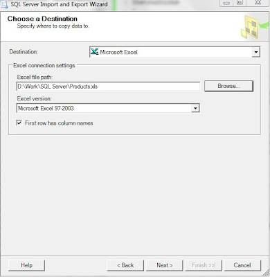
 Step 3: Choose a Destination
 Step 4: Specify Table Copy or Query
 Step 5: Select Source Tables and Views
 Step 6: Review Data Type Mapping
 Step 7: Save and Run Package
 Step 8: Save SSIS Package
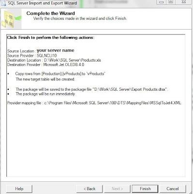
 Step 9: Complete the Wizard
 Step 10: Executing the Package
 If the package run successfully you can go on and check the exported data, apply additional formatting, etc.
 As can be seen the package contains two tasks, the ‘Preparation SQL Task 1’ which creates the table (e.g. vProducts) in the Excel file, and ‘Data Flow Task 1’ which dumps the data in the created table. By double clicking the ‘Data Flow Task 1’ you could see its content:
- the ‘Source - vProducts’ OLEDB Data Source holding the connectivity information to the SQL Server and the list of Columns in scope.
- the ‘Data Conversion’ Transformation that allows converting the data between Source and Destination given the fact that Excel has different data types than SQL Server
- the ‘Destination - vProducts’ Excel Destination holding the connectivity information for the Excel file and the Mappings in place.
 You could explore the properties of each object in order to learn more about its attributes used and the values they took.
 If you haven’t done any changes to the Excel file to which you moved the data (e.g. Products.xls) and haven’t moved the file, then the package will fail when it attempts to run the ‘the ‘Preparation SQL Task 1’ task because a table with the expected name already exists in the file.
 In order to avoid this error to appear you’ll have to delete from the Excel file the sheet (e.g. vProducts) where the data were dumped and save the file. Now you could execute again the package and it should execute without additional issues.


