💎SQL Reloaded: The WINDOW Clause in SQL Server 2022 (Part II: Running Totals)

In the previous post I shown how to use the newly introduced WINDOW clause in SQL Server 2022 by providing some historical context concerning what it took to do the same simple aggregations as SUM or AVG within previous versions of SQL Server. Let's look at another scenario based on the previously created Sales.vSalesOrders view - using the same two functions in providing running totals. 

A running total is a summation of a sequence of values (e.g. OrderQty) ordered by a key, typically one or more columns that uniquely define the sequence, something like a unique record identifier (e.g. SalesOrderId). Moreover, the running total can be defined within a partition (e.g. Year/Month).

In SQL Server 2000, to calculate the running total and average for a value within a partition would resume implementing the logic for each attribute in correlated subqueries. One needed thus one subquery for each attribute, resulting in multiple processing of the base tables. Even if the dataset was already in the memory, it still involves a major overhead.

-- running total/average based on correlated subquery (SQL Server 2000+)
SELECT SOL.SalesOrderId 
, SOL.ProductId
, SOL.OrderDate
, SOL.[Year]
, SOL.[Month]
, SOL.OrderQty
, (-- correlated subquery
  SELECT SUM(SRT.OrderQty)
  FROM Sales.vSalesOrders SRT
  WHERE SRT.ProductId = SOL.ProductId 
    AND SRT.[Year] = SOL.[Year]
	AND SRT.[Month] = SOL.[Month]
	AND SRT.SalesOrderId <= SOL.SalesOrderId
   ) RunningTotalQty
, (-- correlated subquery
  SELECT AVG(SRT.OrderQty)
  FROM Sales.vSalesOrders SRT
  WHERE SRT.ProductId = SOL.ProductId 
    AND SRT.[Year] = SOL.[Year]
	AND SRT.[Month] = SOL.[Month]
	AND SRT.SalesOrderId <= SOL.SalesOrderId
   ) RunningAvgQty
FROM Sales.vSalesOrders SOL
WHERE SOL.ProductId IN (745)
  AND SOL.[Year] = 2012
  AND SOL.[Month] BETWEEN 1 AND 3
ORDER BY SOL.SalesOrderId 

Then SQL Server 2005 allowed consolidating the different correlated subqueries into one by using the CROSS APPLY join:

-- running total/average based on correlated subquery with CROSS APPLY (SQL Server 2005+)
SELECT SOL.SalesOrderId 
, SOL.ProductId
, SOL.OrderDate
, SOL.[Year]
, SOL.[Month]
, SOL.OrderQty
, SRT.RunningTotalQty
, SRT.RunningAvgQty
FROM Sales.vSalesOrders SOL
     CROSS APPLY (-- correlated subquery
	  SELECT SUM(SRT.OrderQty) RunningTotalQty
	  , AVG(SRT.OrderQty) RunningAvgQty
	  FROM Sales.vSalesOrders SRT
	  WHERE SRT.ProductId = SOL.ProductId 
		AND SRT.[Year] = SOL.[Year]
		AND SRT.[Month] = SOL.[Month]
		AND SRT.SalesOrderId <= SOL.SalesOrderId
   ) SRT
WHERE SOL.ProductId IN (745)
  AND SOL.[Year] = 2012
  AND SOL.[Month] BETWEEN 1 AND 3
ORDER BY SOL.SalesOrderId 

Even if SQL Server 2005 introduced window functions that work on a partition, an ORDER BY clause was supported only with SQL Server 2012:

-- running total/average based on window functions (SQL Server 2012+)
SELECT SOL.SalesOrderId 
, SOL.ProductId
, SOL.OrderDate
, SOL.[Year]
, SOL.[Month]
, SOL.OrderQty
, SUM(SOL.OrderQty) OVER (PARTITION BY SOL.ProductId, SOL.[Year], SOL.[Month] ORDER BY SOL.SalesOrderId) RunningTotalQty
, AVG(SOL.OrderQty) OVER (PARTITION BY SOL.ProductId, SOL.[Year], SOL.[Month] ORDER BY SOL.SalesOrderId) RunningAvgQty
FROM Sales.vSalesOrders SOL
WHERE SOL.ProductId IN (745)
  AND SOL.[Year] = 2012
  AND SOL.[Month] BETWEEN 1 AND 3
ORDER BY SOL.SalesOrderId 

Now, in SQL Server 2022 the WINDOW clause allows simplifying the query as follows by defining the partition only once:

-- running total/average based on window functions and clause (SQL Server 2022+)
SELECT SOL.SalesOrderId 
, SOL.ProductId
, SOL.OrderDate
, SOL.[Year]
, SOL.[Month]
, SOL.OrderQty
, SUM(SOL.OrderQty) OVER SalesByMonth AS RunningTotalQty

, AVG(SOL.OrderQty) OVER SalesByMonth AS RunningAvgQty

FROM Sales.vSalesOrders SOL
WHERE SOL.ProductId IN (745)
  AND SOL.[Year] = 2012
  AND SOL.[Month] BETWEEN 1 AND 3
WINDOW SalesByMonth AS (PARTITION BY SOL.ProductId, SOL.[Year], SOL.[Month] ORDER BY SOL.SalesOrderId)
ORDER BY SOL.SalesOrderId 

Moreover, the WINDOW clause allows forward (and backward) referencing of one window into the other:

-- running total/average based on window functions and clause (SQL Server 2022+)
SELECT SOL.SalesOrderId 
, SOL.ProductId
, SOL.OrderDate
, SOL.[Year]
, SOL.[Month]
, SOL.OrderQty
-- simple aggregations
, SUM(SOL.OrderQty) OVER SalesByMonth AS TotalQty

, AVG(SOL.OrderQty) OVER SalesByMonth AS AvgQty

-- running totals
, SUM(SOL.OrderQty) OVER SalesByMonthSorted AS RunningTotalQty

, AVG(SOL.OrderQty) OVER SalesByMonthSorted AS RunningAvgQty

FROM Sales.vSalesOrders SOL
WHERE SOL.ProductId IN (745)
  AND SOL.[Year] = 2012
  AND SOL.[Month] BETWEEN 1 AND 3
WINDOW SalesByMonth AS (PARTITION BY SOL.ProductId, SOL.[Year], SOL.[Month])
, SalesByMonthSorted AS (SalesByMonth ORDER BY SOL.SalesOrderId)
ORDER BY SOL.SalesOrderId 

Happy coding!

💎💫SQL Reloaded: Querying Azure Synapse Metadata for the D365 CRM & FO Tables Exported via Azure Synapse Link for Dataverse

Enabling Azure Synapse Link for Dataverse for Dynamics 365 CRM (D365 CRM) or for Dynamics 365 Finance & Operations (D365 FO) allows to have all the needed tables for reporting in a CDM structure, however the csv files with data don’t have any headers, which makes it challenging to use directly the files without the corresponding metadata. For example, attempting to define external tables would be useless without proper headers and data types. Fortunately, attribute’s name and data types are available in JSON files and can be queried. 

D365 CRM 

For CRM the files start with tables’ names and have the EntityMetadata.json postfix, the files being stored in the Microsoft.Athena.TrickleFeedService folder which lies with the other folders containing the data. Given that all files are in the same folder, the following query can be used to export the metadata for all or some of the tables. Just replace "(container name)" and "(data source)" with the corresponding values for your environment.

 

-- export definition for D365 CRM' CDM (all attributes, all tables)
SELECT DAT.EntityName
, DAT.AttributeName
, DAT.Timestamp
, DAT.AttributeType
, DAT.MetadataId
, DAT.Precision
, DAT.MaxLength
FROM openrowset(
        bulk '/(container name)/Microsoft.Athena.TrickleFeedService/*-EntityMetadata.json',
        data_source = '(data source)',
        format = 'csv',
        fieldterminator ='0x0b',
        fieldquote = '0x0b',
        rowterminator = '0x0b' --> You need to override rowterminator to read classic JSON
    ) with (doc nvarchar(max)) as rows
       CROSS APPLY OPENJSON(doc, '$.AttributeMetadata')--definitions[0].hasAttributes
       with (
         EntityName nvarchar(255) '$.EntityName'
        , AttributeName nvarchar(255) '$.AttributeName'
        , Timestamp nvarchar(50) '$.Timestamp'
        , AttributeType nvarchar(50) '$.AttributeType'
        , MetadataId nvarchar(100) '$.MetadataId'
        , Precision int '$.Precision'
        , MaxLength int '$.MaxLength'
     ) as DAT
WHERE DAT.EntityName IN ('lead', 'opportunity', 'product')

D365 FO 

For Finance & Operations folders’ structure is more complex, a whole hierarchy of folders being built based on a set of predefined categories. One would need to traverse the hierarchy structure to find the files. Thus, it might be easier to generate the metadata for each table. Files’ names start with tables’ names and have the .cdm.json postfix. The below query generates the metadata for the InventTable table. Just replace the "(container name)", "(instance name)" and "(data source)" with the values for your environment.

 

-- export definition for D365 FO's CDM (all attributes, specific table)

SELECT DAT.name
, DAT.dataFormat
FROM openrowset(
        bulk '/(container name)/(instance name)/Tables/SupplyChain/ProductInformationManagement/Main/InventTable.cdm.json',
        data_source = '(data source)',
        format = 'csv',
        fieldterminator ='0x0b',
        fieldquote = '0x0b',
        rowterminator = '0x0b' --> You need to override rowterminator to read classic JSON
    ) with (doc nvarchar(max)) as rows
       CROSS APPLY OPENJSON(doc, '$.definitions[0].hasAttributes')
       with (
          name nvarchar(255) '$.name'
        , dataFormat nvarchar(50) '$.dataFormat'
     ) as DAT

Further Steps

One can obtain thus the needed metadata, however after a first inspection, the data types are too general compared with the ones considered for the data source attributes. One can work probably with these data types as well, though there's a Microsoft recommendation to minimize the row length by using the smallest possible column size, which leads to better query performance. Exporting the metadata from the source system and matching the two datasets based on tables and attributes’ names would allow addressing this recommendation, even if this implies checking from time to time whether their definition changed. The trick is to keep the same sorting order like in the Synapse files. Unfortunately, not all SQL Server data types are supported (e.g. text, ntext, sql_variant, etc.) or are ideal to work with (e.g. money), however there are alternative data types that can be used. 

💎SQL Reloaded: The WINDOW Clause in SQL Server 2022 (Part I: Simple Aggregations)

Between the many new features introduced in SQL Server 2022, Microsoft brings the WINDOW clause for defining the partitioning and ordering of a dataset which uses window functions. But before unveiling the change, let's take a walk down the memory lane.

In the early ages of SQL Server, many of descriptive statistics techniques were resuming in using the averages over a dataset that contained more or less complex logic. For example, to get the total and average of sales per Month, the query based on AdventureWorks database would look something like:

-- aggregated sales orders - detailed (SQL Server 2000+)
SELECT SOL.ProductId
, Year(SOH.OrderDate) [Year]
, Month(SOH.OrderDate) [Month]
, SUM(SOL.OrderQty) TotalQty
, AVG(SOL.OrderQty) AverageQty
FROM Sales.SalesOrderDetail SOL
     JOIN Sales.SalesOrderHeader SOH
	   ON SOL.SalesOrderId = SOH.SalesOrderId
WHERE SOL.ProductId IN (745)
  AND Year(SOH.OrderDate) = 2012
  AND Month(SOH.OrderDate) BETWEEN 1 AND 3
GROUP BY SOL.ProductId
, Year(SOH.OrderDate) 
, Month(SOH.OrderDate)

When possible, the base logic was encapsulated within a view, hiding query's complexity from the users, allowing also reuse and better maintenance, just to mention a few of the benefits of this approach:

-- encapsulating the logic into a view (SQL Server 2000+)
CREATE OR ALTER VIEW Sales.vSalesOrders
AS
-- sales orders details
SELECT SOL.SalesOrderId 
, SOL.ProductId
, Cast(SOH.OrderDate as Date) OrderDate
, Year(SOH.OrderDate) [Year]
, Month(SOH.OrderDate) [Month]
, Cast(SOL.OrderQty as decimal(18,2)) OrderQty
-- many more columns 
FROM Sales.SalesOrderDetail SOL
     JOIN Sales.SalesOrderHeader SOH
	   ON SOL.SalesOrderId = SOH.SalesOrderId
/* -- some constraints can be brought directly into the view
WHERE SOL.ProductId IN (745)
  AND Year(SOH.OrderDate) = 2012
  AND Month(SOH.OrderDate) BETWEEN 1 AND 3
*/

The above query now becomes:

 

-- aggregated sales orders - simplified (SQL Server 2000+)
SELECT SOL.ProductId
, SOL.[Year]
, SOl.[Month]
, SUM(SOL.OrderQty) TotalQty
, AVG(SOL.OrderQty) AverageQty
FROM Sales.vSalesOrders SOL
WHERE SOL.ProductId IN (745)
  AND SOL.[Year] = 2012
  AND SOL.[Month] BETWEEN 1 AND 3
GROUP BY SOL.ProductId
, SOL.[Year]
, SOl.[Month]

In many cases, performing this kind of aggregations was all the users wanted. However, quite often it's useful to look and the individual sales and consider them as part of the broader picture. For example, it would be interesting to know, what's the percentage of an individual value from the total (see OrderQtyPct) or any similar aggregate information. In SQL Server 2000 addressing such requirements would involve a join between the same view - one query with the detailed records, while the other contains the aggregated data:

-- sales orders from the totals (SQL Server 2000+)
SELECT SOL.*
, ASO.TotalQty
, Cast(CASE WHEN ASO.TotalQty <> 0 THEN 100*SOL.OrderQty/ASO.TotalQty ELSE 0 END as decimal(18,2)) OrderQtyPct
, ASO.AverageQty
FROM Sales.vSalesOrders SOL
     JOIN ( -- aggregated sales orders
		SELECT SOL.ProductId
		, SOL.[Year]
		, SOl.[Month]
		, SUM(SOL.OrderQty) TotalQty
		, AVG(SOL.OrderQty) AverageQty
		FROM Sales.vSalesOrders SOL
		WHERE SOL.ProductId IN (745)
		  AND SOL.[Year] = 2012
		  AND SOL.[Month] BETWEEN 1 AND 3
		GROUP BY SOL.ProductId
		, SOL.[Year]
		, SOl.[Month]
	) ASO
	ON SOL.ProductId = ASO.ProductId 
   AND SOL.[Year] = ASO.[Year]
   AND SOL.[Month] = ASO.[Month]
ORDER BY SOL.ProductId
, SOL.OrderDate

Now, just imagine that you can't create a view and having to duplicate the logic each time the view is used! Aggregating the data at different levels would require similar joins to the same view or piece of logic. 

Fortunately, SQL Server 2005 came with two long-awaited features, common table expressions (CTEs) and window functions, which made a big difference. First, CTEs allowed defining inline views that can be referenced multiple times. Secondly, the window functions allowed aggregations within a partition.

 

-- sales orders with CTE SQL Server 2005+ query 
WITH CTE
AS (--sales orders in scope
SELECT SOL.SalesOrderId 
, SOL.ProductId
, Cast(SOH.OrderDate as Date) OrderDate
, Year(SOH.OrderDate) [Year]
, Month(SOH.OrderDate) [Month]
, SOL.OrderQty
FROM Sales.SalesOrderDetail SOL
     JOIN Sales.SalesOrderHeader SOH
	   ON SOL.SalesOrderId = SOH.SalesOrderId
WHERE SOL.ProductId IN (745)
  AND Year(SOH.OrderDate) = 2012
  AND Month(SOH.OrderDate) BETWEEN 1 AND 3
)
SELECT SOL.SalesOrderId 
, SOL.ProductId
, SOL. OrderDate
, SOL.[Year]
, SOL.[Month]
, SOL.OrderQty
, SUM(SOL.OrderQty) OVER(PARTITION BY SOL.[Year], SOL.[Month]) TotalQty
, AVG(SOL.OrderQty)  OVER(PARTITION BY SOL.[Year], SOL.[Month]) AverageQty
FROM CTE SOL
WHERE SOL.ProductId IN (745)
  AND SOL.[Year] = 2012
  AND SOL.[Month] BETWEEN 1 AND 3

This kind of structuring the queries allows to separate the base logic for better maintainability, readability and fast prototyping. Once the logic from CTE becomes stable, it can be moved within a view, following to replace the CTE reference with view's name in the final query. On the other side, the window functions allow writing more flexible and complex code, even if the statements can become occasionally complex (see OrderQtyPct):

 

-- aggregated sales orders (SQL Server 2005+)
SELECT SOL.SalesOrderId 
, SOL.ProductId
, SOL. OrderDate
, SOL.[Year]
, SOL.[Month]
, SOL.OrderQty
, SUM(SOL.OrderQty) OVER(PARTITION BY SOL.[Year], SOL.[Month]) TotalQty
, AVG(SOL.OrderQty)  OVER(PARTITION BY SOL.[Year], SOL.[Month]) AverageQty
, Cast(CASE WHEN SUM(SOL.OrderQty) OVER(PARTITION BY SOL.[Year], SOL.[Month]) <> 0 THEN 100*SOL.OrderQty/SUM(SOL.OrderQty) OVER(PARTITION BY SOL.[Year], SOL.[Month]) ELSE 0 END as decimal(18,2)) OrderQtyPct
FROM Sales.vSalesOrders SOL
WHERE SOL.ProductId IN (745)
  AND SOL.[Year] = 2012
  AND SOL.[Month] BETWEEN 1 AND 3

Now, SQL Server 2022 allows to further simplify the logic by allowing to define with a name the window at the end of the statement and reference the name in several window functions (see last line of the query):

-- Aggregations per month (SQL Server 2022+)
SELECT SOL.SalesOrderId 
, SOL.ProductId
, SOL. OrderDate
, SOL.[Year]
, SOL.[Month]
, SOL.OrderQty
, SUM(SOL.OrderQty) OVER SalesByMonth AS TotalQty
, AVG(SOL.OrderQty) OVER SalesByMonth AS AverageQty
, Cast(CASE WHEN SUM(SOL.OrderQty) OVER SalesByMonth <> 0 THEN 100*SOL.OrderQty/SUM(SOL.OrderQty) OVER SalesByMonth ELSE 0 END as decimal(18,2)) OrderQtyPct
FROM Sales.vSalesOrders SOL
WHERE SOL.ProductId IN (745)
  AND SOL.[Year] = 2012
  AND SOL.[Month] BETWEEN 1 AND 3
WINDOW SalesByMonth AS (PARTITION BY SOL.[Year], SOL.[Month])

Moreover, several windows can be defined. For example, aggregating the data also per year:

-- Aggregations per month and year (SQL Server 2022+) 
SELECT SOL.SalesOrderId 
, SOL.ProductId
, SOL. OrderDate
, SOL.[Year]
, SOL.[Month]
, SOL.OrderQty
, SUM(SOL.OrderQty) OVER SalesByMonth AS TotalQtyByMonth
, AVG(SOL.OrderQty) OVER SalesByMonth AS AverageQtyByMonth
, Cast(CASE WHEN SUM(SOL.OrderQty) OVER SalesByMonth <> 0 THEN 100*SOL.OrderQty/SUM(SOL.OrderQty) OVER SalesByMonth ELSE 0 END as decimal(18,2)) OrderQtyPctByMonth
, SUM(SOL.OrderQty) OVER SalesByYear AS TotalQtyByYear
, AVG(SOL.OrderQty) OVER SalesByYear AS AverageQtyByYear
, Cast(CASE WHEN SUM(SOL.OrderQty) OVER SalesByYear <> 0 THEN 100*SOL.OrderQty/SUM(SOL.OrderQty) OVER SalesByYear ELSE 0 END as decimal(18,2)) OrderQtyPctByYear
FROM Sales.vSalesOrders SOL
WHERE SOL.ProductId IN (745)
  AND SOL.[Year] = 2012
  AND SOL.[Month] BETWEEN 1 AND 3
WINDOW SalesByMonth AS (PARTITION BY SOL.[Year], SOL.[Month])
, SalesByYear AS  (PARTITION BY SOL.[Year])

Isn't that cool? It will take probably some time to get used in writing and reading this kind of queries, though using descriptive names for the windows should facilitate the process! 

As a side note, even if there's no product function like in Excel, there's a mathematical trick to transform a product into a sum of elements by applying the Exp (exponential) and Log (logarithm) functions (see example).

Happy coding!

🛢DBMS: Data Warehouse/Mart (Just the Quotes)

"Unfortunately, just collecting the data in one place and making it easily available isn’t enough. When operational data from transactions is loaded into the data warehouse, it often contains missing or inaccurate data. How good or bad the data is a function of the amount of input checking done in the application that generates the transaction. Unfortunately, many deployed applications are less than stellar when it comes to validating the inputs. To overcome this problem, the operational data must go through a 'cleansing' process, which takes care of missing or out-of-range values. If this cleansing step is not done before the data is loaded into the data warehouse, it will have to be performed repeatedly whenever that data is used in a data mining operation." (Joseph P Bigus,"Data Mining with Neural Networks: Solving business problems from application development to decision support", 1996)

"There are four levels of data in the architected environment - the operational level, the atomic (or the data warehouse) level, the departmental (or the data mart) level, and the individual level. These different levels of data are the basis of a larger architecture called the corporate information factory (CIF). The operational level of data holds application-oriented primitive data only and primarily serves the high-performance transaction-processing community. The data-warehouse level of data holds integrated, historical primitive data that cannot be updated. In addition, some derived data is found there. The departmental or data mart level of data contains derived data almost exclusively. The departmental or data mart level of data is shaped by end-user requirements into a form specifically suited to the needs of the department. And the individual level of data is where much heuristic analysis is done." (William H Inmon, "Building the Data Warehouse" 4th Ed., 2005)

"Having a purposeless or poorly performing dashboard is more common than not. This happens when the underlying architecture is not designed properly to support the needs of dashboard interaction. There is an obvious disconnect between the design of the data warehouse and the design of the dashboards. The people who design the data warehouse do not know what the dashboard will do; and the people who design the dashboards do not know how the data warehouse was designed, resulting in a lack of cohesion between the two. A similar disconnect can also exist between the dashboard designer and the business analyst, resulting in a dashboard that may look beautiful and dazzling but brings very little business value." (Nils H Rasmussen et al, "Business Dashboards: A visual catalog for design and deployment", 2009)

"Having multiple data lakes replicates the same problems that were created with multiple data warehouses - disparate data siloes and data fiefdoms that don't facilitate sharing of the corporate data assets across the organization. Organizations need to have a single data lake from which they can source the data for their BI/data warehousing and analytic needs. The data lake may never become the 'single version of the truth' for the organization, but then again, neither will the data warehouse. Instead, the data lake becomes the 'single or central repository for all the organization's data' from which all the organization's reporting and analytic needs are sourced." (Billl Schmarzo, "Driving Business Strategies with Data Science: Big Data MBA" 1st Ed., 2015)

"There are, however, many problems with independent data marts. Independent data marts: (1) Do not have data that can be reconciled with other data marts (2) Require their own independent integration of raw data (3) Do not provide a foundation that can be built on whenever there are future analytical needs." (William H Inmon & Daniel Linstedt, "Data Architecture: A Primer for the Data Scientist: Big Data, Data Warehouse and Data Vault", 2015)

"Unfortunately, some organizations are replicating the bad data warehouse practice by creating special-purpose data lakes - data lakes to address a specific business need. Resist that urge! Instead, source the data that is needed for that specific business need into an 'analytic sandbox' where the data scientists and the business users can collaborate to find those data variables and analytic models that are better predictors of the business performance. Within the 'analytic sandbox', the organization can bring together (ingest and integrate) the data that it wants to test, build the analytic models, test the model's goodness of fit, acquire new data, refine the analytic models, and retest the goodness of fit." (Billl Schmarzo, "Driving Business Strategies with Data Science: Big Data MBA" 1st Ed., 2015)

"Data quality in warehousing and BI is typically defined in terms of the 4 C’s - is the data clean, correct, consistent, and complete? When it comes to big data, there are two schools of thought that have different views and expectations of data quality. The first school believes that the gold standard of the 4 C’s must apply to all data (big and little) used for clinical care and performance metrics. The second school believes that in big data environments, a stringent data quality standard is impossible, too costly, or not required. While diametrically opposite opinions may play well in panel discussions, they do little to reconcile the realities of healthcare data quality." (Prashant Natarajan et al, "Demystifying Big Data and Machine Learning for Healthcare", 2017) 

"Data warehousing has always been difficult, because leaders within an organization want to approach warehousing and analytics as just another technology or application buy. Viewed in this light, they fail to understand the complexity and interdependent nature of building an enterprise reporting environment." (Prashant Natarajan et al, "Demystifying Big Data and Machine Learning for Healthcare", 2017)

"A data lake is a storage repository that holds a very large amount of data, often from diverse sources, in native format until needed. In some respects, a data lake can be compared to a staging area of a data warehouse, but there are key differences. Just like a staging area, a data lake is a conglomeration point for raw data from diverse sources. However, a staging area only stores new data needed for addition to the data warehouse and is a transient data store. In contrast, a data lake typically stores all possible data that might be needed for an undefined amount of analysis and reporting, allowing analysts to explore new data relationships. In addition, a data lake is usually built on commodity hardware and software such as Hadoop, whereas traditional staging areas typically reside in structured databases that require specialized servers." (Mike Fleckenstein & Lorraine Fellows, "Modern Data Strategy", 2018)

"A data warehouse follows a pre-built static structure to model source data. Any changes at the structural and configuration level must go through a stringent business review process and impact analysis. Data lakes are very agile. Consumption or analytical layer can be modified to fit in the model requirements. Consumers of a data lake are not constant; therefore, schema and modeling lies at the liberty of analysts and scientists." (Saurabh Gupta et al, "Practical Enterprise Data Lake Insights", 2018)

"Data warehousing, as we are aware, is the traditional approach of consolidating data from multiple source systems and combining into one store that would serve as the source for analytical and business intelligence reporting. The concept of data warehousing resolved the problems of data heterogeneity and low-level integration. In terms of objectives, a data lake is no different from a data warehouse. Both are primary advocates of terms like 'single source of truth' and 'central data repository'." (Saurabh Gupta et al, "Practical Enterprise Data Lake Insights", 2018)

"A defining characteristic of the data lakehouse architecture is allowing direct access to data as files while retaining the valuable properties of a data warehouse. Just do both!" (Bill Inmon et al, "Building the Data Lakehouse", 2021)

"The data lakehouse architecture presents an opportunity comparable to the one seen during the early years of the data warehouse market. The unique ability of the lakehouse to manage data in an open environment, blend all varieties of data from all parts of the enterprise, and combine the data science focus of the data lake with the end user analytics of the data warehouse will unlock incredible value for organizations. [...] "The lakehouse architecture equally makes it natural to manage and apply models where the data lives." (Bill Inmon et al, "Building the Data Lakehouse", 2021)

🌡Performance Management: Mastery (Part II: First Time Right - The Aim toward Operational Excellence)

 

Performance Management Series

Rooted in Six Sigma methodology as a step toward operational excellence, First Time Right (FTR) implies that any procedure is performed in the right manner the first time and every time. It equates to minimizing the waste in its various forms (inventory, motion, overprocessing, overproduction, waiting, transportation, defects). Like many quality concepts from the manufacturing industry, the concept was transported in the software development process as principle, process, goal and/or metric. Thus, it became part of Software Engineering, Project Management, Data Science, and any other similar endeavors whose outcome results in software products. 

Besides the quality aspect, FTR is rooted also in the economic imperative – the need to achieve something in the minimum amount of time with the minimum of effort. It’s about being efficient in delivering a product or achieving a given target. It can be associated with continuous improvement, learning and mastery, the aim being to encompass FTR as part of organization’s culture. 

Even if not explicitly declared, FTR lurks in each task planned. It seems that it became common practice to plan with the FTR in mind, however between this theoretical aim and practice there’s as usual an important gap. Unfortunately, planners, managers and even tasks' performers often forget that mistakes are made, that several iterations are needed to get the job done. It starts with the communication between people in clarifying the requirements and ends with the formal sign off. All the deviations from the FTR add up in the deviations between expected and actual effort, though probably more important are the deviations from the plan and all the consequences deriving from it. Especially in complex projects this adds up into a spiral of issues that can easily reinforce themselves. 

Many of the jobs that imply creativity, innovation, research or exploration require at least several iterations to get the job done and this is independent of participants’ professionalism and experience. Moreover, the more quality one needs, the higher the effort, the 80/20 being sometimes a good approximation of the effort needed. In extremis, aiming for perfection instead of excellence can make certain tasks a never-ending story. 

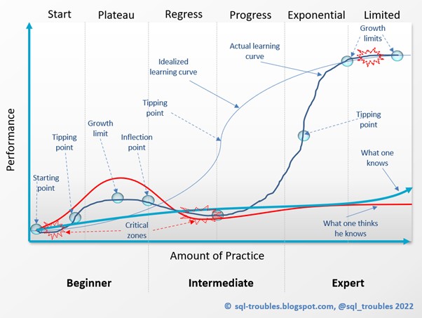
Achieving FTR requires practice - the more novelty, the higher the complexity, the communication or the synchronization needs, the more practice is needed. It starts with the individual to master the individual tasks and ends with the team, where communication, synchronization and other aspects need to be considered. The practice is usually achieved on hands-on work as part of the daily duties, project work, and so on. Unfortunately, it’s based primarily on individual experience, and seldom groomed in advance, as preparation for future tasks. That’s why sometimes when efficiency is needed in performing critical complex tasks, one also needs to consider the learning curve in achieving the required quality. 

Of course, many organizations demand from job applicants experience and, when possible, they hire people with experience, however the diversity, complexity and changing nature of tasks require further practice. This aspect is somehow recognized in the implementation in organizations of the various forms of DevOps, though how many organizations adopt it and enforce it on a regular basis? Moreover, a major requirement of nowadays businesses is to be agile, and besides the mere application of methodologies, being agile means to have also a FTR mindset. 

FTR starts with the wish for mastery at individual and team level and, with the right management attention, by allocating time for learning, self-development in the important areas, providing relevant feedback and building an infrastructure for knowledge sharing and harnessing, FTR can become part of organization’s culture. It’s up to each of us to do it!

💎SQL Reloaded: Successive Price Increases/Discounts via Windowing Functions and CTEs

I was trying today to solve a problem that apparently requires recursive common table expressions, though they are not (yet) available in Azure Synapse serverless SQL pool. The problem can be summarized in the below table definition, in which given a set of Products with an initial Sales price, is needed to apply Price Increases successively for each Cycle. The cumulated increase is simulated in the last column for each line. 

Unfortunately, there is no SQL Server windowing function that allows multiplying incrementally the values of a column (similar as the running total works). However, there’s a mathematical trick that can be used to transform a product into a sum of elements by applying the Exp (exponential) and Log (logarithm) functions (see Solution 1), and which frankly is more elegant than applying CTEs (see Solution 2). 

-- create table with test data
SELECT *
INTO dbo.ItemPrices
FROM (VALUES ('ID001', 1000, 1, 1.02, '1.02')
, ('ID001', 1000, 2, 1.03, '1.02*1.03')
, ('ID001', 1000, 3, 1.03, '1.02*1.03*1.03')
, ('ID001', 1000, 4, 1.04, '1.02*1.03*1.03*1.04')
, ('ID002', 100, 1, 1.02, '1.02')
, ('ID002', 100, 2, 1.03, '1.02*1.03')
, ('ID002', 100, 3, 1.04, '1.02*1.03*1.04')
, ('ID002', 100, 4, 1.05, '1.02*1.03*1.04*1.05')
) DAT (ItemId, SalesPrice, Cycle, PriceIncrease, CumulatedIncrease)

-- reviewing the data
SELECT *
FROM dbo.ItemPrices

-- Solution 1: new sales prices with log & exp
SELECT ItemId
, SalesPrice
, Cycle
, PriceIncrease
, EXP(SUM(Log(PriceIncrease)) OVER(PARTITION BY Itemid ORDER BY Cycle)) CumulatedIncrease
, SalesPrice * EXP(SUM(Log(PriceIncrease)) OVER(PARTITION BY Itemid ORDER BY Cycle)) NewSalesPrice
FROM dbo.ItemPrices

-- Solution 2: new sales prices with recursive CTE
;WITH CTE 
AS (
-- initial record
SELECT ITP.ItemId
, ITP.SalesPrice
, ITP.Cycle
, ITP.PriceIncrease
, cast(ITP.PriceIncrease as decimal(38,6)) CumulatedIncrease
FROM dbo.ItemPrices ITP
WHERE ITP.Cycle = 1
UNION ALL
-- recursice part
SELECT ITP.ItemId
, ITP.SalesPrice
, ITP.Cycle
, ITP.PriceIncrease
, Cast(ITP.PriceIncrease * ITO.CumulatedIncrease as decimal(38,6))  CumulatedIncrease
FROM dbo.ItemPrices ITP
    JOIN CTE ITO
	  ON ITP.ItemId = ITO.ItemId
	 AND ITP.Cycle-1 = ITO.Cycle
)
-- final result
SELECT ItemId
, SalesPrice
, Cycle
, PriceIncrease
, CumulatedIncrease
, SalesPrice * CumulatedIncrease NewSalesPrice
FROM CTE
ORDER BY ItemId
, Cycle


-- validating the cumulated price increases (only last ones)
SELECT 1.02*1.03*1.03*1.04 
, 1.02*1.03*1.04*1.05

-- cleaning up
DROP TABLE IF EXISTS dbo.ItemPrices

Notes:
1. The logarithm in SQL Server’s implementation works only with positive numbers!
2. For simplification I transformed percentages (e.g. 1%) in values that are easier to multitply with (e.g. 1.01). The solution can be easily modified to consider discounts.
3. When CTEs are not available, one is forced to return to the methods used in SQL Server 2000 (I've been there) and thus use temporary tables or table variables with loops. Moreover, the logic can be encapsulated in multi-statement table-valued functions (see example), unfortunately, another feature not (yet) supported by serverless SQL pools. 
4. Unfortunately, STRING_AGG, which concatenates values across rows, works only with a GROUP BY clause. Anyway, its result is useless without the availability of a Eval function in SQL (see example), however the Expr function available in data flows could be used as workaround.
4. Even if I thought about the use of logarithms for transforming the product into a sum, I initially ignored the idea, thinking that the solution would be too complex to implement. So, the credit goes to another blogpost. Kudos!

Happy coding!

🧮ERP: Planning (Part V: It’s all about Partnership II)

When starting an ERP implementation project an organization needs to fill the existing knowledge gaps in respect to whatever it takes to achieve the goals associated with the respective project. Therefore, it makes sense to work with a implementer that can help cover the gaps directly or indirectly. Moreover, it makes sense to establish a long-term relationship that would allow to harness ERP system’s capabilities after project’s end, increase the ROI and, why not, find other areas of cooperation. It’s in theory what a partner does, and a strategic technology partnership is about – providing any kind of technological expertise the customer doesn't have in-house. 

Unfortunately, from being a ‘service provider’ to becoming a ‘partner’ is a challenging road for many organizations, especially when this type of relationship is not understood and managed accordingly. Partnership’s management may resume in defining common goals, principles, values and processes, establishing a communication strategy and a common understanding of the challenges and the steps ahead, providing visibility into the cost estimates, billing, resources’ availability and utilization. Addressing these aspects would offer a framework on which the partnerships can nourish. Without considering these topics, the implementer remains just a 'service provider', no matter of the names used to characterize the relationship. 

Now, the use of the word ‘partner’ would make someone think that only one partner is considered, typically a big to middle-sized organization that would have this kind of resources. The main reason behind this reasoning is that the number of functional areas and volume of skillset required for filling the requirements of an implementation are high compared with other projects, the resources needing to be available on-demand without affecting the other constraints: costs, quality, time. This can be challenging, therefore can be met scenarios in which two or more external organizations are involved in the partnership, ideally organizations that complement each other. 

It is common in ERP implementations to appeal also to individual consultants for specific areas or the whole project. The principles and values of a partnership, as well the framework behind, can be applied to individual consultants as well. Independently of resources’ provenience more important is the partnership ‘mindset’ - being together in the same boat, working together on a shared and understood strategy, with clear goals and objectives.

Moreover, the people participating in the project must have a ‘partner's mindset’ as well. Without this, the project will likely get different impulses in the wrong direction(s), as a group’s interests will take priority over the ones of the organization. Ideally, this mindset should extend to the whole organization as topics like Data Quality and Process Improvement must be an organization’s effort, deeply imprinted in organization’s culture.

More like ever, it’s important for the business to see and treat the IT department as a ‘partner’ and not as a ‘service provider’ by providing the needed level of transparency in requirements, issues, practices and processes, by treating the IT department as equal party in the decision-making and addressing its current and future strategical requirements. Ideally, this partnership should happen long before the implementation starts, given that it takes time for mentalities and practices to change, for knowledge to be acquired and used appropriately. 

Building a partnership takes time, effort and strategic thinking, this on top of the actual implementation, increasing thus the overall complexity, at least at the beginning. Does it pay off? Like in a marriage, it’s useful to have somebody you can trust, who knows you, whom you can rely upon, and talk with to find solutions. However, only time will tell whether such expectations are met and kept till the end. 

Previous <||> Next