18 April 2023

📊Graphical Representation: Graphics We Live By I (The Analytics Marathon)

Graphical Representation
Graphical Representation Series

In a diagram adapted from an older article [1], Brent Dykes, the author of "Effective Data Storytelling" [2], makes a parallel between Data Analytics and marathon running, considering that an organization must pass through the depicted milestones, the percentages representing how many organizations reach the respective milestones:


It's a nice visualization and the metaphor makes sense given that running a marathon requires a long-term strategy to address the gaps between the current and targeted physical/mental form and skillset required to run a marathon, respectively for approaching a set of marathons and each course individually. Similarly, implementing a Data Analytics initiative requires a Data Strategy supposed to address the gaps existing between current and targeted state of art, respectively the many projects run to reach organization's goals. 

It makes sense, isn't it? On the other side the devil lies in details and frankly the diagram raises several questions when is compared with practices and processes existing in organizations. This doesn't mean that the diagram is wrong, just that it doesn't seem to reflect entirely the reality. 

The percentages represent author's perception of how many organizations reach the respective milestones, probably in an repeatable manner (as there are several projects). Thus, only 10% have a data strategy, 100% collect data, 80% of them prepare the data, while at the opposite side only 15% communicate insight, respectively 5% act on information.

Considering only the milestones the diagram looks like a funnel and a capability maturity model (CMM). Typically, the CMMs are more complex than this, evolving with technologies' capabilities. All the mentioned milestones have a set of capabilities that increase in complexity and that usually help differentiated organization's maturity. Therefore, the model seems too simple for an actual categorization.  

Typically, data collection has a specific scope resuming to surveys, interviews and/or research. However, the definition can be extended to the storage of data within organizations. Thus, data collection as the gathering of raw data is mainly done as part of their value supporting processes, and given the degree of digitization of data, one can suppose that most organizations gather data for the different purposes, even if only a small part are maybe digitized.

Even if many organizations build data warehouses, marts, lakehouses, mashes or whatever architecture might be en-vogue these days, an important percentage of the reporting needs are covered by standard reports or reporting tools that access directly the source systems without data preparation or even data visualization. The first important question is what is understood by data analytics? Is it only the use of machine learning and statistical analysis? Does it resume only to pattern and insight finding or does it includes also what is typically considered under the Business Intelligence umbrella? 

Pragmatically thinking, Data Analytics should consider BI capabilities as well as its an extension of the current infrastructure to consider analytic capabilities. On the other side Data Warehousing and BI are considered together by DAMA as part of their Data Management methodology. Moreover, organizations may have a Data Strategy and a BI strategy, respectively a Data Analytics strategy as they might have different goals, challenges and bodies to support them. To make it even more complicated, an organization might even consider all these important topics as part of the Data or even Information Governance, or consider BI or Analytics without Data Management. 

So, a Data Strategy might or might not address Data Analytics at all. It's a matter of management philosophy, organizational structure, politics and other factors. Probably, having a strayegy related to data should count. Even if a written and communicated data-related strategy is recommended for all medium to big organizations, only a small percentage of them have one, while small organizations might ignore the topic completely.

At least in the past, data analysis and its various subcomponents was performed before preparing and visualizing the data, or at least in parallel with data visualization. Frankly, it's a strange succession of steps. Or does it refers to exploratory data analysis (EDA) from a statistical perspective, which requires statistical experience to model and interpret the facts? Moreover, data exploration and discovery happen usually in the early stages.

The most puzzling step is the last one - what does the author intended with it? Ideally, data should be actionable, at least that's what one says about KPIs, OKRs and other metrics. Does it make sense to extend Data Analytics into the decision-making process? Where does a data professional's responsibilities end and which are those boundaries? Or does it refer to the actions that need to be performed by data professionals? 

The natural step after communicating insight is for the management to take action and provide feedback. Furthermore, the decisions taken have impact on the artifacts built and a reevaluation of the business problem, assumptions and further components is needed. The many steps of analytics projects are iterative, some iterations affecting the Data Strategy as well. The diagram shows the process as linear, which is not the case.

For sure there's an interface between Data Analytics and Decision-Making and the processes associated with them, however there should be clear boundaries. E.g., it's a data professional's responsibility to make sure that the data/information is actionable and eventually advise upon it, though whether the entitled people act on it is a management topic. Not acting upon an information is also a decision. Overstepping boundaries can put the data professional into a strange situation in which he becomes responsible and eventually accountable for an action not taken, which is utopic.

The final question - is the last mile representative for the analytical process? The challenge is not the analysis and communication of data but of making sure that the feedback processes work and the changes are addressed correspondingly, that value is created continuously from the data analytics infrastructure, that data-related risks and opportunities are addressed as soon they are recognized. 

As any model, a diagram doesn't need to be correct to be useful and might not be even wrong in the right context and argumentation. A data analytics CMM might allow better estimates and comparison between organizations, though it can easily become more complex to use. Between the two models lies probably a better solution for modeling the data analytics process.

Resources:
[1] Brent Dykes (2022) "Data Analytics Marathon: Why Your Organization Must Focus On The Finish", Forbes (link)
[2] Brent Dykes (2019) Effective Data Storytelling: How to Drive Change with Data, Narrative and Visuals (link)

16 April 2023

🔖Book Review: Willard C Brinton's Graphic Methods for Presenting Facts (1919)

"It is often with impotent exasperation that a person having the knowledge sees some fallacious conclusion accepted, or some wrong policy adopted, just because known facts cannot be marshalled and presented in such manner as to be effective." 

This is the conclusion phrase from the first paragraph of Willard C Brinton's "Graphic Methods for Presenting Facts", in which the author expresses his disappointment about the impossibility of bridging the important gap existing between data collection and presentation on side, and the decision-making on the other. Despite being written more than a century ago (1915), the issue seems to be so actual, the average data professional probably met this kind of situation at least once in a lifetime, if not on a regular basis. 

I found out about this book from Bridget Cogley & Vidya Setlur's "Functional Aesthetics for Data Visualization" (2020), which credits Brinton for "shaping the path toward broad use of charts". I found a digitized copy of the book at Internet Archive and browsing though it I found it appealing for a deeper reading and a first review. 

Written in a simple style stripped of any mathematical or statistical formulae, and thus approachable by the average nontechnical reader, the book addresses the techniques and challenges of graphical authors in preparing charts and other graphical content for their consumption in organizations for insight and decision-making, as well for the masses. It mentions also the projecting of graphs as lantern slides to accompany a talk, a precursor of nowadays' forms of presentations.

The engineering and statistical background of the author can be seen in the meticulosity with which the book was written. The book discusses the graphic methods for presenting facts in graphical form, which are the component parts and how can be used to attract readers' attention, respectively present them in an effective manner. Several principle-like statements are considered though the book and listed together in the last chapters, rules that can be found in modern books as well, though probably less exemplified. 

From organization charts to maps, from circle and bar charts to time plots, the number and variety of graphical displays is overwhelming and at the same time surprising for a book that old, especially when we consider the publishing technologies available. As mentioned by the author, color printing of the book was prohibitive given the costs, only one ink color being used. However, this doesn't diminish the quality of visuals considered. Compared with nowadays' books, which seem to attempt compensating the lack of novelty with too much color and mentions of technologies, book's graphics stand out in their simplicity and richness of exemplifications. It is sad to remark that the graphical displays are better chosen and the book is better written than some of nowadays books on data visualization.

Comparing the language and vocabulary used nowadays with the one used then, the reader can see the difficulties of approaching a subject found in its early years, the author recognizing the lack of standards and the difficulties of showing quantitative facts in true proportions. It's also true that more modern authors like Tufte or Cleveland were facing same challenge 70 years later. 

About the author is worth mentioning that he was chairman of the "Joint Committee on Standards for Graphic Presentation" initiated in 1913, committee that published in 1915 their first brief report which consisted of 17 simply basic rules, a first attempt of standardizing the principles of graphic presentation. In 1939 Brinton published a second book on "Graphic Presentation", with less text and abundant colorful graphical displays. Even if some charts are available in the second book as well, overall, the two books seem to complement each other and should be a lecture for the data professional as well for the average reader interested in understanding the use of graphical methods.

Previous Post <<||>>  Next Post

References:
[1] Willard C Brinton, "Graphic Methods for Presenting Facts", 1919 (link)
[2] Bridget Cogley & Vidya Setlur, "Functional Aesthetics for Data Visualization" (2020)
[3] Willard C Brinton, "Graphic Presentation", 1939 (link)
[4] Joint Committee on Standards for Graphic Presentation, "Publications of the American Statistical Association" Vol.14 (112), 1915 (Jstor)

03 March 2023

🧊Data Warehousing: Architecture (Part IV: Building a Modern Data Warehouse with Azure Synapse)

Data Warehousing

Introduction

When building a data warehouse (DWH) several key words or derivatives of them appear in requirements: secure, flexible, simple, scalable, reliable, performant, non-redundant, modern, automated, real-timed, etc. As it proves in practice, all these requirements are sometimes challenging to address with the increased complexity of the architecture chosen. There are so many technologies on the DWH market promising all these at low costs, low effort and high ROI, though DWH projects continue to fail addressing the business and technical requirements.

On a basic level for building a DWH is needed a data storage layer and an ETL (Extract, Transfer, Load) tool responsible for the data movement between the various source systems and DWH, and eventually within the DWH itself. After that, each technology added to the landscape tends to increase the overall complexity (and should be regarded with a critical eye in what concerns the advantages and disadvantages).

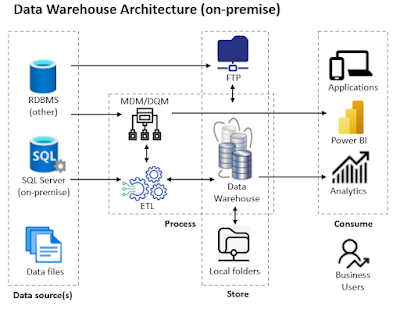
Data Warehouse Architecture (on-premise)

A Reference Architecture

When building a DWH or a data migration solution, which has many of the characteristics of a DWH, from the many designs, I prefer to keep things as simple as possible.  An approach based on a performant database engine like SQL Server as storage layer and SSIS (SQL Server Integration Services) as ETL proved to be the best choice until now, allowing to address most of the technical requirements by design. Then come the choices on how and where to import and transform the data, at what level of granularity, on how the semantic layer is built, how the data are accessed, etc.

Being able to pull (see extract subprocess) the data from the data sources on a need by basis offers the most flexible approach, however there are cases in which the direct access to source data is not possible, having to rely on a push approach, where data are dumped regularly to a given location (e.g. FTP folder structure), following to be picked up as needed. It's actually a hybrid between a push and pull, because a fully push approach would mean pushing the data directly to the DWH, which can be also acceptable, though might offer lower control on data's movement and involve a few other challenges (e.g. permissions, concurrency). 

Data can be prepared for the DWH in the source systems (e.g. exposed via data objects or API calls), anywhere in between via ETL-based transformations (see transform subprocess) or directly in the DWH. I prefer importing the data (see load subprocess) 1:1 without any transformations from the various sources via SSIS (or similar technologies) into a set of tables that designated the staging area. It's true that in this way the ETL technology is used to a minimum, though unless there's a major benefit to use it for data transformations, using DWH's capabilities and SQL for data processing can provide better performance and flexibility

Besides the selection of the columns in scope (typically columns with meaningful values), it's important not to do any transformations in the extraction layer because the data is imported faster (eventually using fast load options as in SSIS) and it assures a basis for troubleshooting (as the data don't change between loads). Some filters can be applied only when the volume of data is high, and the subset of the data could be identified clearly (e.g. when data are partitioned based on a key like business unit, legal entity or creation date).

For better traceability, the staging schemas can reflect the systems they come from, the tables and the columns should have the same names, respectively same data types. On such tables no constraints are applied and no indexes are needed. They can be constructed however on the production tables (aka base tables) - copy of the tables from production. 

Some DWH architects try replicating the constraints from the source systems and/or add more constraints on top to define the various business rules. Rigor is good in some scenarios, though it can involve a considerable effort and it might be challenging to keep over time, especially when considering the impact of big data on DWH architectures. Instead of using constraints, building a set of SQL scripts that pinpoint the issues as reports allow more flexibility with the risk of having inconsistencies running wild through the reports. The data should be cleaned in the source system and not possible then properly addressed in the DWH. Applying constraints will make the data unavailable for reporting until data are corrected, while being more permissive would allow dirty data. Thus, either case has advantages or disadvantages, though the latter seems to be more appropriate. 

Indexes on the production schema should reflect the characteristics of the queries run on the data and shouldn't replicate the indexes from the source environments, even if some overlaps might exist. In practice, dropping the non-clustered indexes on the production tables before loading the data from staging, and recreating them afterwards proves to provide faster loading (see load optimization techniques). 

The production tables are used for building a "semantic" data model or something similar. Several levels of views, table-valued functions and/or indexed/materialized views allows building the dimensions and facts tables, the latter incorporating the business logic needed by the reports. Upon case, stored-procedures, physical or temporary tables, table variables can be used to prepare the data, though they tend to break the "free" flow of data as steps in-between need to be run. On the other side, in certain scenarios their use is unavoidable. 

The first level of views (aka base views) is based on the base tables without any joins, though they include only the fields in use (needed by the business) ordered and "grouped" together based on their importance or certain characteristics. The views can include conversions of data types, translations of codes into meaningful values, and quite seldom filters on the data. Based on these "base" views the second level is built, which attempts to define the dimension and fact tables at the lowest granularity. These views include joins between tables coming from the same or different systems, respectively mappings of values defined in tables, and whatever it takes to build such entities. However, transformations on individual fields are pushed, when possible, to the lower level to minimize logic redundancy. From similar reasons, the logic could be broken down over two or more "helper" views when visible benefits could be obtained from it (e.g troubleshooting, reuse, maintenance). It's important to balance between creating too many helper views and encapsulating too much logic in a view. 

One of the design principles used in building the entities is to minimize the redundance of the fields used, ideally without having columns duplicated between entities at this level. This would facilitate the traceability of columns to the source tables within the "semantic" layer (typically in the detriment of a few more joins). In practice, one is forced to replicate some columns to simplify some parts of the logic. 

Further views can be built based on the dimension and fact entities to define the logic needed by the reports. Only these objects are used and no direct reference to the "base" tables or views are made. Moreover, to offer better performance when the views can be materialized or, when there's an important benefit, physically saved as table (e.g. having multiple indexes for different scenarios). It's the case of entities with considerable data volume called over and over. 

This approach of building the entities is usually flexible enough to address most of the reporting requirements, independently whether the technical solution has the characteristics of a DWH, data mart or data migration layer. Moreover, the overall architectural approach can be used on-premise as well in cloud architectures, where Azure SQL Server and ADF (Azure Data Factory) provide similar capabilities. Compared with standard SQL Server, some features might not be available, while other features might bring further benefits, though the gaps should be neglectable.

Data Management topics like Master Data Management (MDM), Data Quality Management (DQM) and/or Metadata Management can be addressed as well by using third-party tools or tools from the Microsoft stack - Master Data Services (MDS) and Data Quality Services (DQS) in combination with SSIS help addressing a wide range of scenarios - however these are optional. 

Moving to the Cloud

Within the context of big data, characterized by (high/variable) volume, value, variety, velocity, veracity, and further less important V's, the before technical requirements still apply, however within a cloud environment the overall architecture becomes more complex. Each component becomes a service. There are thus various services for data ingestion, storage, processing, sharing, collaboration, etc. The way data are processed involves also several important transformations: ETL becomes ELT, FTP and local storage by Data Lakes, data packages by data pipelines, stateful by stateless, SMP (Symmetric Multi-Processing) by MPP (Massive Parallel Processing), and so on.

As file storage is less expensive than database storage, there's an increasing trend of dumping business critical data into the Data Lake via data pipelines or features like Link to Data Lake or Export to Data Lake (*), which synchronize the data between source systems and Data Lake in near real-time at table or entity level. Either saved as csv, parquet, delta lake or any other standard file format, in single files or partitions, the data can be used directly or indirectly for analytics.

Cloud-native warehouses allow addressing topics like scalability, elasticity, fault-tolerance and performance by design, though further challenges appear as compute needs to be decoupled from storage, the workloads need to be estimated for assuring the performance, data may be distributed across data centers spanning geographies, the infrastructure is exposed to attacks, etc. 

Azure Synapse

If one wants to take advantage of the MPP architecture's power, Microsoft provides an analytical architecture based on Azure Synapse, an analytics service that brings together data integration, enterprise DWH, and big data analytics. Besides two types of SQL-based data processing services  (dedicated vs serverless SQL pools) it comes also with a Spark pool for in-memory cluster computing.

A DWH based on Azure Synapse is not that different from the reference architecture described above for an on-premise solution. Actually, a DWH based on a dedicated SQL pool (aka a physical data warehouse) involves the same steps mentioned above. 
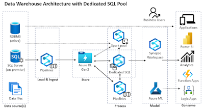
Data Warehouse Architecture with Dedicated SQL Pool

The data can be imported via ETL/ELT pipelines in the DWH, though there are also mechanisms for consuming the data directly from the files stored in the Data Lake or Azure storage. CETAS (aka Create External Table as Select) can be defined on top of the data files, the external tables acting as "staging" or "base" tables in the architecture described above. When using a dedicated SQL pool it makes sense to use the CETAS as "staging" tables, the processed data following to be dumped to "optimized" physical tables for consumption and refreshed periodically. However, when this happens the near real-time character of data is lost. Using the CETAs as base tables would keep this characteristic as long the data isn't saved physically in tables or files, maybe in the detriment of performance.

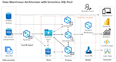
Using a dedicated SQL pool for direct reporting can become expensive as the pool needs to be available at least during business hours for incoming user requests, or at least for importing the data and refreshing the datasets. When using the CETAS as a base table, a serverless (aka on-demand) SQL pool, which uses a per-pay-use billing model could prove to be more cost-effective and flexible in many scenarios. By design, it helps to keep the near real-time character of the data. Moreover, even if the data are actually moved from the source tables into the Data Lake, this architecture has the characteristics of a logical data warehouse:

Data Warehouse Architecture with Serverless SQL Pool

Unfortunately, unless one uses Spark tables, misuses views or adds an Azure SQL database to the architecture, there are no physical tables or materialized views in a serverless SQL pool. There's still the option to use data pipelines for regullarly exporting intermediary data to files (incl. over partitions or folders), even if this involves more overhead as it's not possible to export data over SQL syntax to files more than once (though this might change in the future). For certain scenario it could be useful to store data in a Azure SQL Server or similar database, including a dedicated SQL pool. 

Choosing between serverless and dedicated SQL pool is not an exclusive choice, both or all 3 types of pools (if we consider also the Spark pool) can be used in the architecture for addressing specific challenges, especially when we consider that there are important differences between the features available in each of the pools. Moreover, one can start the PoC based on the serverless SQL pool and when the solution became mature enough and used in all enterprise, parts of the logic or all of it can be migrated to a dedicated SQL pool. This would allow to save costs at the beginning in the detriment of further effort later. 

Talking about the physical storage, data engineers recommend defining within a Data Lake several layers (aka regions, zones) labeled as bronze, silver and gold (and probably platinum will join the club anytime soon). The bronze layer refers to the raw data available in the Data Lake, including the files on which the initial CETAS are defined upon. The silver refers to transformed, cleaned, enriched and integrated data, data resulting from the second layer of views described above. The gold layer refers to the data to which business logic was applied and prepared for consumption, data resulting from the final layer of views. Of course, data pipelines can be used to prepare the data at these stages, though a view-based approach offers more flexibility, are easier to troubleshoot, manage and reuse than data pipelines.

Ideally the gold data should involve no or minimal further transformation before reaching the users, though that's not realistic. Building a DWH takes a considerable time and the business can't usually wait until everything is in place. Therefore, reports based on DWH will continue to coexist with reports directly accessing the source data, which will lead to controversies. Enforcing a single source of truth will help to minimize the gap, though will not eliminate it completely. 

Closing Notes

These are just outlines of a minimal reference architecture. There's more to consider, as there are several alternatives (see [1] [2] [3] [4]) for each of the steps considered in here, each technology, new features or mechanisms opening new opportunities. The advantages and disadvantages should be always considered against the business needs and requirements. One approach, even if recommended, might not work for all, though unless there's an important requirement or an opportunity associated with an additional technology, deviating from reference architectures might not be such a good idea afterall.

Note:
(*) Existing customers have until 1-Nov-2024 to transition from Export to Data lake to Synapse link. Microsoft advises new customers to use Synapse Link. 


Resources:
[1] Microsoft Learn (2022) Modern data warehouse for small and medium business (link)
[2] Microsoft Learn (2022) Data warehousing and analytics (link)
[3] Microsoft Learn (2022) Enterprise business intelligence (link)
[4] Microsoft Learn (2022) Serverless Modern Data Warehouse Sample using Azure Synapse Analytics and Power BI (link)
[5] Coursera (2023) Data Warehousing with Microsoft Azure Synapse Analytics (link) [course, free to audit]
[6] SQLBits (2020) Mahesh Balija's Building Modern Data Warehouse with Azure Synapse Analytics (link)
[7] Matt How (2020) The Modern Data Warehouse in Azure: Building with Speed and Agility on Microsoft’s Cloud Platform (Amazon)
[8] James Serra's blog (2022) Data lake architecture (link)
[9] SQL Stijn (2022) SQL Building a Modern Lakehouse Data Warehouse with Azure Synapse Analytics: Moving your Database to the lake (link)
[10] Solliance (2022) Azure Synapse Analytics Workshop 400 (link) [GitHub repository]

22 February 2023

💎🏭SQL Reloaded: Automatic Statistics Creation & Dropping for CETAS based on CSV File Format in Serverless SQL Pool

Introduction

The serverless SQL pool query optimizer uses statistics to calculate and compare the cost of various query plans, and then choose the plan with the lowest cost. Automatic creation of statistics is turned on for parquet file format, though for CSV file format statistics will be automatically created only when OPENROWSET is used. This means that when creating CETAS based on CSV the statistics need to be created manually. 

This would be one more reason for holding the files in the Data Lake as parquet files. On the other side there are also many files already available in CSV format, respectively technoloqies that allows exporting data only/still as CSV. Moreover, transforming the files as parquet is not always technically feasible.

Using OPENROWSET could also help, though does it make sense to use a different mechanismus for the CSV file format? In some scenarios will do. I prefer to have a unitary design, when possible. Moreover, even if some columns are not needed, they can still be useful for certain scenarios (e.g. troubleshooting, reevaluating their use, etc.). 

There are files, especially the ones coming from ERPs (Enterprise Resource Planning) or similar systems, which have even a few hundred columns (on average between 50 and 100 columns). Manually creating  the statistics for the respective tables will cost lot of time and effort. To automate the process there are mainly three choices:
(1) Creating statistics for all the columns for a given set of tables (e.g. for a given schema).
(2) Finding a way to automatically identify the columns which are actually used.
(3) Storing the list of tables and columns on which statistics should be build (however the list needs to be maintained manually). 

Fortunately, (1) can be solved relatively easy, based on the available table metadata, however it's not the best solution, as lot of statistics will be unnecessarily created. (2) is possible under certain architectures or additional effort. (3) takes time, though it's also an approachable solution.

What do we need?

For building the solution, we need table and statistics metadata, and the good news is that the old SQL Server queries still work. To minimize code's repetition, it makes sense to encapsulate the logic in views. For table metadata one can use the sys.objects DMV as is more general (one can replace sys.objects with sys.tables to focus only on tables):

-- drop the view (for cleaning)
-- DROP VIEW IF EXISTS dbo.vAdminObjectColumns

-- create view
CREATE OR ALTER VIEW dbo.vObjectColumns
AS 
-- object-based column metadata
SELECT sch.name + '.' + obj.name two_part_name
, sch.Name schema_name
, obj.name object_name
, col.name column_name
, obj.type
, CASE 
	WHEN col.is_ansi_padded = 1 and LEFT(udt.name , 1) = 'n' THEN col.max_length/2
	ELSE col.max_length
  END max_length
, col.precision 
, col.scale
, col.is_nullable 
, col.is_identity
, col.object_id
, col.column_id
, udt.name as data_type
, col.collation_name
, ROW_NUMBER() OVER(PARTITION BY col.object_id ORDER BY col.column_id) ranking FROM sys.columns col JOIN sys.types udt on col.user_type_id= udt.user_type_id JOIN sys.objects obj ON col.object_id = obj.object_id JOIN sys.schemas as sch on sch.schema_id = obj.schema_id -- testing the view SELECT obc.* FROM dbo.vObjectColumns obc WHERE obc.object_name LIKE '<table name>%' AND obc.schema_name = 'CRM' AND obc.type = 'U' ORDER BY obc.two_part_name , Ranking

The view can be used also as basis for getting the defined stats:

-- drop the view (for cleaning)
-- DROP VIEW IF EXISTS dbo.vAdminObjectStats

-- create view 
CREATE OR ALTER VIEW dbo.vObjectStats
AS
-- object-based column statistics
SELECT obc.two_part_name + '.' + QuoteName(stt.name) three_part_name
, obc.two_part_name
, obc.schema_name
, obc.object_name
, obc.column_name
, stt.name stats_name
, STATS_DATE(stt.[object_id], stt.stats_id) AS last_updated
, stt.auto_created
, stt.user_created
, stt.no_recompute
, stt.has_filter 
, stt.filter_definition
, stt.is_temporary 
, stt.is_incremental 
, stt.auto_drop 
, stt.stats_generation_method_desc
, stt.[object_id]
, obc.type 
, stt.stats_id
, stc.stats_column_id
, stc.column_id
FROM dbo.vObjectColumns obc
     LEFT JOIN sys.stats_columns stc 
	   ON stc.object_id = obc.object_id
	  AND stc.column_id = obc.column_id 
          LEFT JOIN sys.stats stt
            ON stc.[object_id] = stt.[object_id] 
           AND stc.stats_id = stt.stats_id

-- testing the view 
SELECT * FROM dbo.vObjectStats obs WHERE (obs.auto_created = 1 OR obs.user_created = 1) AND obs.type = 'U' AND obs.object_name = '<table name>' ORDER BY obs.two_part_name , obs.column_id

Now we have a basis for the next step. However, before using the stored procedure define below, one should use the last query and check whether statistics were defined before on a table. Use for testing also a table for which you know that statistics are available.

Create Statistics

The code below is based on a similar stored procedure available in the Microsoft documentation (see [1]). It uses a table's column metadata, stores them in a temporary table and then looks through each record, create the DDL script and runs it:

-- drop procedure (for cleaning)
--DROP PROCEDURE dbo.pCreateStatistics

-- create stored procedure
CREATE OR ALTER PROCEDURE dbo.pCreateStatistics
(   @schema_name nvarchar(50)
,   @table_name nvarchar(100)
)
AS
-- creates statistics for serverless SQL pool
BEGIN
	DECLARE @query as nvarchar(1000) = ''
	DECLARE @index int = 1, @nr_records int = 0

	-- drop temporary table if it exists 
	DROP TABLE IF EXISTS #stats_ddl;

	-- create temporary table 
	CREATE TABLE #stats_ddl( 
	  schema_name nvarchar(50)
	, table_name nvarchar(128)
	, column_name nvarchar(128)
	, ranking int
	);

	-- fill table
	INSERT INTO #stats_ddl
	SELECT obc.schema_name
	, obc.object_name
	, obc.column_name 
	, ROW_NUMBER() OVER(ORDER BY obc.schema_name, obc.object_name) ranking
	FROM dbo.vObjectColumns obc
	WHERE obc.type = 'U' -- tables
	  AND IsNull(@schema_name, obc.schema_name) = obc.schema_name 
	  AND IsNull(@table_name, obc.object_name) = obc.object_name

	SET @nr_records = (SELECT COUNT(*) FROM #stats_ddl)

	WHILE @index <= @nr_records
	BEGIN
		SET @query = (SELECT 'CREATE STATISTICS '+ QUOTENAME('stat_' + schema_name + '_' + table_name + '_' + column_name) + ' ON '+ QUOTENAME(schema_name) + '.' + QUOTENAME(table_name) + '(' + QUOTENAME(column_name) + ')' 
			   FROM #stats_ddl ddl
			   WHERE ranking = @index);

		BEGIN TRY
		        -- execute ddl
			EXEC sp_executesql @query;
		END TRY
		BEGIN CATCH
			SELECT 'create failed for ' + @query;
		END CATCH

		SET @index+=1;
	END

	DROP TABLE #stats_ddl;
END


-- test stored procedure (various scenario)
EXEC dbo.pCreateStatistics '<schema name>', '<table name>' -- based on schema & table
EXEC dbo.pCreateStatistics '<schema name>', NULL -- based on a schema
EXEC dbo.pCreateStatistics NULL, '<table name>' -- based on a table

Notes:
IMPORTANT!!! I recommend testing the stored procedure in a test environment first for a few tables and not for a whole schema. If there are too many tables, this will take time.

Please note that rerunning the stored procedure without deleting previously the statitics on the tables in scope will make the procedure raise failures for each column (behavior by design), though the error messages can be surpressed by commenting the code, if needed. One can introduce further validation, e.g. considering only the columns which don't have a statistic define on them.

Further Steps?

What can we do to improve the code? It would be great if we could find a way to identify the columns which are used in the queries. It is possible to retrieve the queries run in serverless SQL pool, however identifying the tables and columns from there or a similar source is not a straightforward solution. 

The design of views based on the external tables can help in the process! I prefer to build on top of the external tables a first level of views (aka "base views") that include only the fields in use (needed by the business) ordered and "grouped" together based on their importance or certain characteristics. The views are based solely on the external table and thus contain no joins. They can include conversions of data types, translations of codes into meaningful values, and quite seldom filters on the data. However, for traceability the name of the columns don't change! This means that if view's name is easily identifiable based on external table's name, we could check view's columns against the ones of the external table and create statistics only for the respective columns. Using a unique prefix (e.g. "v") to derive views' name from tables' name would do the trick.

To do that, we need to create a view that reflects the dependencies between objects (we'll be interested only in external tables vs views dependencies):

-- drop view (for cleaning)
-- DROP VIEW IF EXISTS dbo.vObjectsReferenced

-- create view
CREATE OR ALTER VIEW dbo.vObjectsReferenced
AS 
-- retrieving the objects referenced 
SELECT QuoteName(sch.name) + '.' + QuoteName(obj.name) AS two_part_name 
, obj.object_id 
, obj.schema_id 
, sch.name schema_name 
, obj.name object_name 
, obj.type
, QuoteName(scr.name) + '.'+ QuoteName(sed.referenced_entity_name) AS ref_two_part_name 
, obr.object_id ref_object_id
, obj.schema_id ref_schema_id 
, scr.name ref_schema_name 
, obr.name ref_object_name 
, obr.type ref_type
FROM sys.sql_expression_dependencies sed 
     JOIN sys.objects obj
       ON obj.object_id = sed.referencing_id 
	      JOIN sys.schemas as sch
	        ON obj.schema_id = sch.schema_id 
	 JOIN sys.objects obr
	   ON sed.referenced_id = obr.object_id
	      JOIN sys.schemas as scr
	        ON obr.schema_id = scr.schema_id

-- testing the view
SELECT top 10 *
FROM dbo.vObjectsReferenced
WHERE ref_type = 'U'

With this, the query used above to fill the table becomes:

-- fill table query with column selection 
SELECT obc.schema_name
, obc.object_name
, obc.column_name 
, ROW_NUMBER() OVER(ORDER BY obc.schema_name, obc.object_name) ranking
FROM dbo.vObjectColumns obc
WHERE obc.type = 'U' -- tables
	AND IsNull(@schema_name, obc.schema_name) = obc.schema_name 
	AND IsNull(@table_name, obc.object_name) = obc.object_name
	AND EXISTS ( -- select only columns referenced in views
	    SELECT * 
		FROM dbo.vObjectsReferenced obr 
		    JOIN dbo.vAdminObjectColumns obt
			ON obr.object_id = obt.object_id 
		WHERE obt.type = 'V' -- view
		AND obr.object_name  =  'v' + obr.ref_object_name
		AND obc.object_id = obr.ref_object_id
		AND obc.column_name = obt.column_name);

This change will reduce the number of statistics created on average by 50-80%. Of course, there will be also cases in which further statistics need to be added manually. One can use this as input for an analysis of the columns used and store the metadata in a file, do changes to it and base on it statistics' creation. 

Drop Statistics

Dropping the indexes resumes to using the dbo.vObjectStats view created above for the schema and/or table provided as parameter. The logic is similar to statistics' creation:

-- drop stored procedure (for cleaning)
-- DROP PROCEDURE IF EXISTS dbo.pDropStatistics

-- create procedure
CREATE OR ALTER PROCEDURE dbo.pDropStatistics
(   @schema_name nvarchar(50)
,   @table_name nvarchar(128)
)
AS
-- drop statistics for a schema and/or external table in serverless SQL pool
BEGIN

	DECLARE @query as nvarchar(1000) = ''
	DECLARE @index int = 1, @nr_records int = 0

	-- drop temporary table if it exists 
	DROP TABLE IF EXISTS #stats_ddl;

	-- create temporary table 
	CREATE TABLE #stats_ddl( 
	 three_part_name nvarchar(128)
	, ranking int
	);

	-- fill table
	INSERT INTO #stats_ddl
	SELECT obs.three_part_name
	, ROW_NUMBER() OVER(ORDER BY obs.three_part_name) ranking
	FROM dbo.vObjectStats obs
	WHERE obs.type = 'U' -- tables
	  AND IsNull(@schema_name, obs.schema_name) = obs.schema_name 
	  AND IsNull(@table_name, obs.object_name) = obs.object_name

	SET @nr_records = (SELECT COUNT(*) FROM #stats_ddl)

	WHILE @index <= @nr_records
	BEGIN
   
		SET @query = (SELECT 'DROP STATISTICS ' + ddl.three_part_name
			   FROM #stats_ddl ddl
			   WHERE ranking = @index);

		BEGIN TRY
		        -- execute ddl
			EXEC sp_executesql @query;
		END TRY
		BEGIN CATCH
			SELECT 'drop failed for ' + @query;
		END CATCH

		SET @index+=1;
	END

	DROP TABLE #stats_ddl;
END

Note:
IMPORTANT!!!
I recommend testing the stored procedure in a test environment first for a few tables and not for a whole schema. If there are too many tables, this will take time.

Closing Thoughts

The solution for statistics' creation is not perfect, though it's a start! It would have been great if such a feature would be provided by Microsoft, and probably they will, given the importance of statistics of identifying an optimal plan. It would be intersting to understand how much statistics help in a distributed environment and what's the volume of data processed for this purpose. 

Please let me know if you found other workarounds for statistics's automation.

Happy coding!

Previous Post  <<||>>  Next Post

References:
[1] Microsoft Learn (2022) Statistics in Synapse SQL (link)

11 February 2023

💎SQL Reloaded: Misusing Views in Serverless SQL Pool

The lack of user-defined tables in serverless SQL pool is probably one of the biggest gaps one needs to overcome as developer in Azure Synapse. On the other side, given that views are "virtual tables", views can be misused to store small chunks of data that don't change that often. 

In the process there are two activities involved - preparing the data, respectively creating the view. Some developers might prefer preparing the data in Excel though, when possible, I prepare the data directly from the source system. For example, the first four columns from the below query can be used for the first approach, while the last column prepares the data as needed by a VALUES.

-- Product subcategories denormalized
SELECT PCT.ProductSubcategoryID
, PCT.ProductCategoryID
, PSC.Name Category
, PCT.Name Subcategory 
, CONCAT(', (''', PCT.ProductSubcategoryID, ''', ''', PCT.ProductCategoryID, ''', ''', PSC.Name, ''', ''', PCT.Name, ''')') [Values] 
FROM Production.ProductSubcategory PCT
     JOIN Production.ProductCategory PSC
	   ON PCT.ProductCategoryID = PSC.ProductCategoryID

Independently of the method used for data preparation, the view can be built as follows:

-- creating the view
CREATE VIEW dbo.ProductCategories
AS
-- Product categories
SELECT Cast(DAT.ProductSubcategoryID as int) ProductSubcategoryID
, Cast(DAT.ProductCategoryID as int) ProductCategoryID
, Cast(DAT.Category as nvarchar(255)) Category
, Cast(DAT.Subcategory  as nvarchar(255)) Subcategory
, Dense_Rank() OVER (PARTITION BY DAT.Category, DAT.Subcategory 
         ORDER BY DAT.ProductSubcategoryID, DAT.ProductCategoryID) Ranking
FROM (-- prepared data
VALUES ('1', '1', 'Bikes', 'Mountain Bikes')
, ('2', '1', 'Bikes', 'Road Bikes')
, ('3', '1', 'Bikes', 'Touring Bikes')
, ('4', '2', 'Components', 'Handlebars')
, ('5', '2', 'Components', 'Bottom Brackets')
, ('6', '2', 'Components', 'Brakes')
) DAT(ProductSubcategoryID, ProductCategoryID, Category, Subcategory)

-- testing the view
SELECT *
FROM dbo.ProductCategories

Observe that for each column was defined explicitly a data type and, even if the definition might change, it's still a better idea than relying on the database engine for inferring the data type. Secondly, I prefer to include also a "Ranking" column based on some attributes I'm expecting to be unique over the whole dataset. This, just in case some duplicate might make its way into the dataset. This is not a must, but something to consider in exceptional cases. 

The alternative would be to save the same data into a file and make it available as a CETAS. For small datasets the overhead can be minimal. This can be a better idea if the users need to modify the data manually. On the other side, storing the definition of a view into an SQL file and making corrections as needed can prove to be faster for a developer, at least until the dataset stabilizes and less changes are needed.

It's important to understand that in this way a feature is misused and there are more likely some penalties deriving from it. As mentioned in the beginning, the dataset must be small (e.g. maximum a few hundreds of records) and change seldom. In extremis, it's not advisable to build a solution based on this!

One scenario I had to use this option was creating a dataset based on recursive logic built inside of a stored procedure, which would output the data in the form needed by the view, as done above. This was used as workaround, as I couldn't save the data via a pipeline. (I had a deja vu from the first attempts of exporting data in SSIS 2005!)

In theory the maintenance of such a view can be automated via a pipeline, if the effort makes sense, and the solution is stable enough. 

I blogged some years back on Misusing Views and Pseudo-Constants.

Happy coding!

Related Posts Plugin for WordPress, Blogger...

About Me

My photo
Koeln, NRW, Germany
IT Professional with more than 24 years experience in IT in the area of full life-cycle of Web/Desktop/Database Applications Development, Software Engineering, Consultancy, Data Management, Data Quality, Data Migrations, Reporting, ERP implementations & support, Team/Project/IT Management, etc.