Showing posts sorted by relevance for query Azure Synapse. Sort by date Show all posts

03 March 2023

🧊Data Warehousing: Architecture (Part IV: Building a Modern Data Warehouse with Azure Synapse)

Data Warehousing

Introduction

When building a data warehouse (DWH) several key words or derivatives of them appear in requirements: secure, flexible, simple, scalable, reliable, performant, non-redundant, modern, automated, real-timed, etc. As it proves in practice, all these requirements are sometimes challenging to address with the increased complexity of the architecture chosen. There are so many technologies on the DWH market promising all these at low costs, low effort and high ROI, though DWH projects continue to fail addressing the business and technical requirements.

On a basic level for building a DWH is needed a data storage layer and an ETL (Extract, Transfer, Load) tool responsible for the data movement between the various source systems and DWH, and eventually within the DWH itself. After that, each technology added to the landscape tends to increase the overall complexity (and should be regarded with a critical eye in what concerns the advantages and disadvantages).
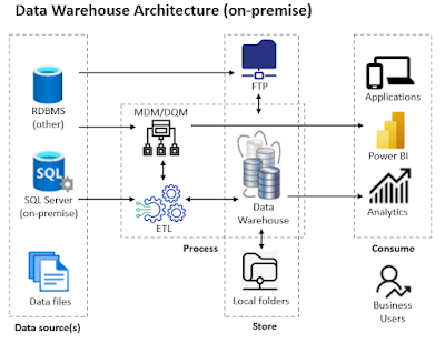
Data Warehouse Architecture (on-premise)

A Reference Architecture

When building a DWH or a data migration solution, which has many of the characteristics of a DWH, from the many designs, I prefer to keep things as simple as possible.  An approach based on a performant database engine like SQL Server as storage layer and SSIS (SQL Server Integration Services) as ETL proved to be the best choice until now, allowing to address most of the technical requirements by design. Then come the choices on how and where to import and transform the data, at what level of granularity, on how the semantic layer is built, how the data are accessed, etc.

Being able to pull (see extract subprocess) the data from the data sources on a need by basis offers the most flexible approach, however there are cases in which the direct access to source data is not possible, having to rely on a push approach, where data are dumped regularly to a given location (e.g. FTP folder structure), following to be picked up as needed. It's actually a hybrid between a push and pull, because a fully push approach would mean pushing the data directly to the DWH, which can be also acceptable, though might offer lower control on data's movement and involve a few other challenges (e.g. permissions, concurrency). 

Data can be prepared for the DWH in the source systems (e.g. exposed via data objects or API calls), anywhere in between via ETL-based transformations (see transform subprocess) or directly in the DWH. I prefer importing the data (see load subprocess) 1:1 without any transformations from the various sources via SSIS (or similar technologies) into a set of tables that designated the staging area. It's true that in this way the ETL technology is used to a minimum, though unless there's a major benefit to use it for data transformations, using DWH's capabilities and SQL for data processing can provide better performance and flexibility

Besides the selection of the columns in scope (typically columns with meaningful values), it's important not to do any transformations in the extraction layer because the data is imported faster (eventually using fast load options as in SSIS) and it assures a basis for troubleshooting (as the data don't change between loads). Some filters can be applied only when the volume of data is high, and the subset of the data could be identified clearly (e.g. when data are partitioned based on a key like business unit, legal entity or creation date).

For better traceability, the staging schemas can reflect the systems they come from, the tables and the columns should have the same names, respectively same data types. On such tables no constraints are applied and no indexes are needed. They can be constructed however on the production tables (aka base tables) - copy of the tables from production. 

Some DWH architects try replicating the constraints from the source systems and/or add more constraints on top to define the various business rules. Rigor is good in some scenarios, though it can involve a considerable effort and it might be challenging to keep over time, especially when considering the impact of big data on DWH architectures. Instead of using constraints, building a set of SQL scripts that pinpoint the issues as reports allow more flexibility with the risk of having inconsistencies running wild through the reports. The data should be cleaned in the source system and not possible then properly addressed in the DWH. Applying constraints will make the data unavailable for reporting until data are corrected, while being more permissive would allow dirty data. Thus, either case has advantages or disadvantages, though the latter seems to be more appropriate. 

Indexes on the production schema should reflect the characteristics of the queries run on the data and shouldn't replicate the indexes from the source environments, even if some overlaps might exist. In practice, dropping the non-clustered indexes on the production tables before loading the data from staging, and recreating them afterwards proves to provide faster loading (see load optimization techniques). 

The production tables are used for building a "semantic" data model or something similar. Several levels of views, table-valued functions and/or indexed/materialized views allows building the dimensions and facts tables, the latter incorporating the business logic needed by the reports. Upon case, stored-procedures, physical or temporary tables, table variables can be used to prepare the data, though they tend to break the "free" flow of data as steps in-between need to be run. On the other side, in certain scenarios their use is unavoidable. 

The first level of views (aka base views) is based on the base tables without any joins, though they include only the fields in use (needed by the business) ordered and "grouped" together based on their importance or certain characteristics. The views can include conversions of data types, translations of codes into meaningful values, and quite seldom filters on the data. Based on these "base" views the second level is built, which attempts to define the dimension and fact tables at the lowest granularity. These views include joins between tables coming from the same or different systems, respectively mappings of values defined in tables, and whatever it takes to build such entities. However, transformations on individual fields are pushed, when possible, to the lower level to minimize logic redundancy. From similar reasons, the logic could be broken down over two or more "helper" views when visible benefits could be obtained from it (e.g troubleshooting, reuse, maintenance). It's important to balance between creating too many helper views and encapsulating too much logic in a view. 

One of the design principles used in building the entities is to minimize the redundance of the fields used, ideally without having columns duplicated between entities at this level. This would facilitate the traceability of columns to the source tables within the "semantic" layer (typically in the detriment of a few more joins). In practice, one is forced to replicate some columns to simplify some parts of the logic. 

Further views can be built based on the dimension and fact entities to define the logic needed by the reports. Only these objects are used and no direct reference to the "base" tables or views are made. Moreover, to offer better performance when the views can be materialized or, when there's an important benefit, physically saved as table (e.g. having multiple indexes for different scenarios). It's the case of entities with considerable data volume called over and over. 

This approach of building the entities is usually flexible enough to address most of the reporting requirements, independently whether the technical solution has the characteristics of a DWH, data mart or data migration layer. Moreover, the overall architectural approach can be used on-premise as well in cloud architectures, where Azure SQL Server and ADF (Azure Data Factory) provide similar capabilities. Compared with standard SQL Server, some features might not be available, while other features might bring further benefits, though the gaps should be neglectable.

Data Management topics like Master Data Management (MDM), Data Quality Management (DQM) and/or Metadata Management can be addressed as well by using third-party tools or tools from the Microsoft stack - Master Data Services (MDS) and Data Quality Services (DQS) in combination with SSIS help addressing a wide range of scenarios - however these are optional. 

Moving to the Cloud

Within the context of big data, characterized by (high/variable) volume, value, variety, velocity, veracity, and further less important V's, the before technical requirements still apply, however within a cloud environment the overall architecture becomes more complex. Each component becomes a service. There are thus various services for data ingestion, storage, processing, sharing, collaboration, etc. The way data are processed involves also several important transformations: ETL becomes ELT, FTP and local storage by Data Lakes, data packages by data pipelines, stateful by stateless, SMP (Symmetric Multi-Processing) by MPP (Massive Parallel Processing), and so on.

As file storage is less expensive than database storage, there's an increasing trend of dumping business critical data into the Data Lake via data pipelines or features like Link to Data Lake or Export to Data Lake (*), which synchronize the data between source systems and Data Lake in near real-time at table or entity level. Either saved as csv, parquet, delta lake or any other standard file format, in single files or partitions, the data can be used directly or indirectly for analytics.

Cloud-native warehouses allow addressing topics like scalability, elasticity, fault-tolerance and performance by design, though further challenges appear as compute needs to be decoupled from storage, the workloads need to be estimated for assuring the performance, data may be distributed across data centers spanning geographies, the infrastructure is exposed to attacks, etc. 

Azure Synapse

If one wants to take advantage of the MPP architecture's power, Microsoft provides an analytical architecture based on Azure Synapse, an analytics service that brings together data integration, enterprise DWH, and big data analytics. Besides two types of SQL-based data processing services  (dedicated vs serverless SQL pools) it comes also with a Spark pool for in-memory cluster computing.

A DWH based on Azure Synapse is not that different from the reference architecture described above for an on-premise solution. Actually, a DWH based on a dedicated SQL pool (aka a physical data warehouse) involves the same steps mentioned above. 
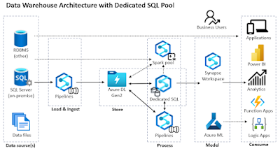
Data Warehouse Architecture with Dedicated SQL Pool

The data can be imported via ETL/ELT pipelines in the DWH, though there are also mechanisms for consuming the data directly from the files stored in the Data Lake or Azure storage. CETAS (aka Create External Table as Select) can be defined on top of the data files, the external tables acting as "staging" or "base" tables in the architecture described above. When using a dedicated SQL pool it makes sense to use the CETAS as "staging" tables, the processed data following to be dumped to "optimized" physical tables for consumption and refreshed periodically. However, when this happens the near real-time character of data is lost. Using the CETAs as base tables would keep this characteristic as long the data isn't saved physically in tables or files, maybe in the detriment of performance.

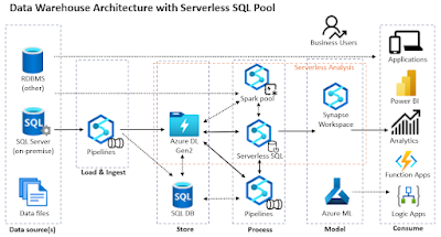
Using a dedicated SQL pool for direct reporting can become expensive as the pool needs to be available at least during business hours for incoming user requests, or at least for importing the data and refreshing the datasets. When using the CETAS as a base table, a serverless (aka on-demand) SQL pool, which uses a per-pay-use billing model could prove to be more cost-effective and flexible in many scenarios. By design, it helps to keep the near real-time character of the data. Moreover, even if the data are actually moved from the source tables into the Data Lake, this architecture has the characteristics of a logical data warehouse:

Data Warehouse Architecture with Serverless SQL Pool

Unfortunately, unless one uses Spark tables, misuses views or adds an Azure SQL database to the architecture, there are no physical tables or materialized views in a serverless SQL pool. There's still the option to use data pipelines for regullarly exporting intermediary data to files (incl. over partitions or folders), even if this involves more overhead as it's not possible to export data over SQL syntax to files more than once (though this might change in the future). For certain scenario it could be useful to store data in a Azure SQL Server or similar database, including a dedicated SQL pool. 

Choosing between serverless and dedicated SQL pool is not an exclusive choice, both or all 3 types of pools (if we consider also the Spark pool) can be used in the architecture for addressing specific challenges, especially when we consider that there are important differences between the features available in each of the pools. Moreover, one can start the PoC based on the serverless SQL pool and when the solution became mature enough and used in all enterprise, parts of the logic or all of it can be migrated to a dedicated SQL pool. This would allow to save costs at the beginning in the detriment of further effort later. 

Talking about the physical storage, data engineers recommend defining within a Data Lake several layers (aka regions, zones) labeled as bronze, silver and gold (and probably platinum will join the club anytime soon). The bronze layer refers to the raw data available in the Data Lake, including the files on which the initial CETAS are defined upon. The silver refers to transformed, cleaned, enriched and integrated data, data resulting from the second layer of views described above. The gold layer refers to the data to which business logic was applied and prepared for consumption, data resulting from the final layer of views. Of course, data pipelines can be used to prepare the data at these stages, though a view-based approach offers more flexibility, are easier to troubleshoot, manage and reuse than data pipelines.

Ideally the gold data should involve no or minimal further transformation before reaching the users, though that's not realistic. Building a DWH takes a considerable time and the business can't usually wait until everything is in place. Therefore, reports based on DWH will continue to coexist with reports directly accessing the source data, which will lead to controversies. Enforcing a single source of truth will help to minimize the gap, though will not eliminate it completely. 

Closing Notes

These are just outlines of a minimal reference architecture. There's more to consider, as there are several alternatives (see [1] [2] [3] [4]) for each of the steps considered in here, each technology, new features or mechanisms opening new opportunities. The advantages and disadvantages should be always considered against the business needs and requirements. One approach, even if recommended, might not work for all, though unless there's an important requirement or an opportunity associated with an additional technology, deviating from reference architectures might not be such a good idea afterall.

Note:
(*) Existing customers have until 1-Nov-2024 to transition from Export to Data lake to Synapse link. Microsoft advises new customers to use Synapse Link. 


Resources:
[1] Microsoft Learn (2022) Modern data warehouse for small and medium business (link)
[2] Microsoft Learn (2022) Data warehousing and analytics (link)
[3] Microsoft Learn (2022) Enterprise business intelligence (link)
[4] Microsoft Learn (2022) Serverless Modern Data Warehouse Sample using Azure Synapse Analytics and Power BI (link)
[5] Coursera (2023) Data Warehousing with Microsoft Azure Synapse Analytics (link) [course, free to audit]
[6] SQLBits (2020) Mahesh Balija's Building Modern Data Warehouse with Azure Synapse Analytics (link)
[7] Matt How (2020) The Modern Data Warehouse in Azure: Building with Speed and Agility on Microsoft’s Cloud Platform (Amazon)
[8] James Serra's blog (2022) Data lake architecture (link)
[9] SQL Stijn (2022) SQL Building a Modern Lakehouse Data Warehouse with Azure Synapse Analytics: Moving your Database to the lake (link)
[10] Solliance (2022) Azure Synapse Analytics Workshop 400 (link) [GitHub repository]

02 March 2024

🧭Business Intelligence: Microsoft Releases for the BI Technology Stack (Timeline)

Business Intelligence
Business Intelligence Series

I started some years back to put together a timeline for the most important events happening in the BI technology stack (work in progress):

2023: Microsoft announces Microsoft Fabric (>>)

  • Synapse Data Warehouse is the next generation of data warehousing in Microsoft Fabric with native support for the delta lake.
  • Data Engineering & Data Science workloads with support for lakehouses, notebooks, Spark Job definitions, models and experiments.
  • Real-Time Analytics is a robust platform tailored to deliver real-time data insights and observability analytics capabilities for a wide range of data types.
  • OneLake provides a single unified storage location for all your data analytics needs.

2022: Microsoft releases SQL Server 2022 (>>)

  • Synapse Link for SQL Server 2022 allows to seamlessly replicate operational data in near real-time to be able to have more powerful analytics.
  • Purview is a unified data governance and management service.

2019: Microsoft launches Azure Synapse Analytics service (formerly SQL Data Warehouse), a limitless analytics service, that brings together enterprise data warehousing and Big Data analytics. (>>)

2019: Microsoft releases SQL Server 2019 (>>)

  •  Big Data Clusters add-in for SQL Server allows to deploy scalable clusters of SQL Server, Spark, and HDFS containers running on Kubernetes (feature to be retired)

2018: Microsoft extends PowerQuery with ETL capabilities. (>>)

2018: Microsoft releases Azure Data Studio, a data management tool that enables to work with SQL Server, Azure SQL DB and SQL DW from Windows, macOS and Linux. (>>)

2017: Microsoft releases Power BI Report Server, an on-premises server that enables Power BI Pro users to publish Power BI reports and distribute them broadly across the enterprise, without requiring report consumers to be licensed individually per use (>>)

2017: Microsoft released SQL Server Data Tools (SSDT), which uses PowerQuery to import and prepare data in SSAS/AAS tabular models.

2017: Microsoft releases SQL Server 2017. (>>)

  • SSRS is no longer available to install through SQL Server setup.
  • Python support added, R Services renamed to Machine Learning Services. (>>)

2016: Microsoft releases SQL Server 2016 (What's new, >>)

  • Query Store allows to monitor and troubleshoot performance issues.
  • SQL Server R Services integrate the R programming language into SQL Server.
  • Direct Query for SSAS.
  • PolyBase for querying the data stored in HDFS. (>>)
  • Support for Support for HDFS in SSIS.
  • Azure SQL Data Warehouse is GA. (>>)
  • modern reports with SSRS. (>>)
  • Real-Time Operational Analytics. (>>)
2016: SQL Server 2014 Developer Edition becomes free. (>>)

2015: Microsoft announces elastic databases SQL Data Warehouse & Azure Data Lake. (>>)

  • Elastic databases allows to build SaaS applications to manage large numbers of databases that have unpredictable resource demand.
  •  Azure SQL Data Warehouse is an elastic data warehouse in the cloud that can dynamically grow, shrink and pause compute in seconds independent of storage.
  • Azure Data Lake is a hyper-scale data store for big data analytic workloads.

2015: Microsoft releases Power BI to the general public.

  • Power BI Designer renamed to Power BI Desktop.
2015: Microsoft releases several Azure services:
  • launches the SQL Server Cloud database.
  • Azure Data Factory (ADF), a fully managed service that does information production by orchestrating data with processing services as managed data pipelines. (>>)
  • Azure Stream Analytics, a fully managed stream processing engine that is designed to analyze and process large volumes of streaming data with sub-millisecond latencies. (>>)

2014: Microsoft released Power BI Designer unifying Power Query, Power Pivot & Power View.

2013: Microsoft announces Power BI for Office 365. (>>)

2012: Microsoft releases with SQL Server 2012. (>>)

  • BI Semantic Model for SSAS provides a single, scalable model for BI applications.
  • Parallel Data Warehouse with PolyBase capabilities. 
  • in-memory capabilities. (>>)
  • Windows Azure SQL Reporting service available (>>)
  • SQL Server Data Tools unifies SQL Server and cloud SQL Azure development for both professional database and application developers.

2010: Microsoft released 

  • Power Pivot as part of SQL Server R2.
  • Azure SQL Database.

2010: Microsoft releases SQL Server 2008 R2.

  • Master Data Services.
  • Power Pivot & Self-service BI capabilities in SSAS.

2008: Microsoft releases SQL Server 2008 (>>)

  • Table compression.
  • Change Data Capture (CDC).

2005: Microsoft releases SQL Server 2005

  • a greatly enhanced version of Analysis Services.
  • SQL Server Integration Services to replace DTS.

2004: Microsoft released SQL Server Reporting Services (SSRS) as add-on to SQL Server 2000.

2000: Microsoft released SQL Server Analysis Services (SSAS) with SQL Server 2000.

1998: Microsoft released SQL Server 7.

  • OLAP services & first MDX specifications.
  • Data Transformation Services (DTS) for ETL workloads.

15 January 2023

💎🏭SQL Reloaded: Monitoring the Synapse serverless SQL pool with Dynamics Management Views I

I feel sometimes flying blind when I build or troubleshoot SQL queries and I don't have the query plan and/or further statistics to understand how the database engine works, why some queries take longer than expected, etc. Unfortunately, Synapse serverless SQL pool doesn't seem to support showing exection plans in SQL Server Management Studio as per now (SHOWPLAN_XML is not supported for SET). I looked at my old queries based on the the sys.dm_exec_requests and sys.dm_exec_query_stats  DMVs, however the results didn't proved to be what I was searching for. (

This weekend, I found Sidney Cirqueira's post on monitoring Synapse serverless SQL pools where he describes how to do that via the Monitoring hub, DMVs, QPI library, respectively Log Analytics. (You should check regularly the Azure Synapse Analytics Blog as it's full of goodies!)

Thus, I found out that there's a new DMV called sys.dm_exec_requests_history which provides at least the duration and the volume of data processes by each statement run on the service:

-- Azure Serverless SQL pool: requests' history 
SELECT top 100 ERH.status
, ERH.transaction_Id
, ERH.distributed_statement_Id 
, ERH.query_hash 
, ERH.login_name 
, ERH.start_time
, ERH.end_time 
, ERH.command 
, ERH.query_text 
--, ERH.total_elapsed_time_ms
, ERH.total_elapsed_time_ms/1000.0 total_elapsed_time_sec
--, ERH.data_processed_mb
, ERH.data_processed_mb/1028.0 data_processed_gb
, ERH.error
, ERH.error_code 
FROM sys.dm_exec_requests_history ERH
ORDER BY ERH.data_processed_mb DESC

It isn't much information, compared with the columns returned by sys.dm_exec_requests, but it's something to start with. At least it allows focusing on the queries with the longest duration (use the above query sorting the records based on the total_elapsed_time_ms descending) or highest volume of data processed:

-- Azure Serverless SQL pool: queries with most data processed
SELECT TOP 50 ERH.query_text  
, COUNT(*) no_runs
, SUM(ERH.total_elapsed_time_ms) total_elapsed_time_ms
, SUM(ERH.data_processed_mb) data_processed_mb
, SUM(ERH.data_processed_mb/1028.0) data_processed_gb
, MIN(ERH.start_time) first_run_date
, MAX(ERH.start_time) last_run_date
FROM sys.dm_exec_requests_history ERH
GROUP BY ERH.query_text
HAVING COUNT(*)>1
ORDER BY data_processed_mb DESC

The same query can be slightly changed to retrieve the volume of data processed by month:
 
-- Azure Serverless SQL pool: data processed by month
SELECT Convert(nvarchar(7), ERH.start_time, 23) [period]
, COUNT(*) no_runs
, SUM(ERH.total_elapsed_time_ms) total_elapsed_time_ms
, SUM(ERH.data_processed_mb) data_processed_mb
, SUM(ERH.data_processed_mb/1028.0) data_processed_gb
, MIN(ERH.start_time) first_run_date
, MAX(ERH.start_time) last_run_date
FROM sys.dm_exec_requests_history ERH
GROUP BY Convert(nvarchar(7), ERH.start_time, 23)
HAVING COUNT(*)>1
ORDER BY data_processed_mb DESC

One can add in the grouping also the login name to break down the analysis by the login that issued the query. Organization's domain can be used to differentiate between system or organization-baed queries.

The volume of data processed is stored also in the sys.dm_external_data_processed DMV aggregated for the current day, week, respectively month as part of the cost control related feature:
 
-- Azure Serverless SQL pool: volume of data processed
SELECT type 
, data_processed_mb 
, data_processed_mb/1028.0 data_processed_gb
FROM sys.dm_external_data_processed

And here's how the output looks like:
 
typedata_processed_mbdata_processed_gb
daily2300.223735
weekly3770.366731
monthly223522217.433852

Notes:
1) I still need to play with the DMVs to understand their scope and limitations.
2) The view appears also in the list of DMVs I idenfitied to be supported the by Synapse serverless SQL pool. As I discoered later, 3 more DMVs are available with useful statistics.
3) The queries based on sys.dm_exec_requests and sys.dm_exec_query_stats DMVs seem to return only the running query based on them.  (Actually, the DMVs seem to work.)
4) The view is available also in SQL Server 2022, though it doesn't seem to be used.
5) According to the above-mentioned source, the view is provided for ticket purposes to help customers better troubleshooting the SQL requests. Use the distributed_statement_id in the tickets raised with Microsoft to troubleshoot any issues with Synapse.
6) Unfortunately, also the useful Query Store feature is not yet supported, even if the DMVs related to it seem to be available. Attempting to enable it results in the error:
"Msg 15869, Level 16, State 9, Line 1
QUERY_STORE is not supported for ALTER DATABASE"

Happy coding!

30 October 2022

💎💫SQL Reloaded: Querying Azure Synapse Metadata for the D365 CRM & FO Tables Exported via Azure Synapse Link for Dataverse

Enabling Azure Synapse Link for Dataverse for Dynamics 365 CRM (D365 CRM) or for Dynamics 365 Finance & Operations (D365 FO) allows to have all the needed tables for reporting in a CDM structure, however the csv files with data don’t have any headers, which makes it challenging to use directly the files without the corresponding metadata. For example, attempting to define external tables would be useless without proper headers and data types. Fortunately, attribute’s name and data types are available in JSON files and can be queried. 

D365 CRM 

For CRM the files start with tables’ names and have the EntityMetadata.json postfix, the files being stored in the Microsoft.Athena.TrickleFeedService folder which lies with the other folders containing the data. Given that all files are in the same folder, the following query can be used to export the metadata for all or some of the tables. Just replace "(container name)" and "(data source)" with the corresponding values for your environment.
 
-- export definition for D365 CRM' CDM (all attributes, all tables)
SELECT DAT.EntityName
, DAT.AttributeName
, DAT.Timestamp
, DAT.AttributeType
, DAT.MetadataId
, DAT.Precision
, DAT.MaxLength
FROM openrowset(
        bulk '/(container name)/Microsoft.Athena.TrickleFeedService/*-EntityMetadata.json',
        data_source = '(data source)',
        format = 'csv',
        fieldterminator ='0x0b',
        fieldquote = '0x0b',
        rowterminator = '0x0b' --> You need to override rowterminator to read classic JSON
    ) with (doc nvarchar(max)) as rows
       CROSS APPLY OPENJSON(doc, '$.AttributeMetadata')--definitions[0].hasAttributes
       with (
         EntityName nvarchar(255) '$.EntityName'
        , AttributeName nvarchar(255) '$.AttributeName'
        , Timestamp nvarchar(50) '$.Timestamp'
        , AttributeType nvarchar(50) '$.AttributeType'
        , MetadataId nvarchar(100) '$.MetadataId'
        , Precision int '$.Precision'
        , MaxLength int '$.MaxLength'
     ) as DAT
WHERE DAT.EntityName IN ('lead', 'opportunity', 'product')

D365 FO
 

For Finance & Operations folders’ structure is more complex, a whole hierarchy of folders being built based on a set of predefined categories. One would need to traverse the hierarchy structure to find the files. Thus, it might be easier to generate the metadata for each table. Files’ names start with tables’ names and have the .cdm.json postfix. The below query generates the metadata for the InventTable table. Just replace the "(container name)", "(instance name)" and "(data source)" with the values for your environment.
 
-- export definition for D365 FO's CDM (all attributes, specific table)
SELECT DAT.name
, DAT.dataFormat
FROM openrowset(
        bulk '/(container name)/(instance name)/Tables/SupplyChain/ProductInformationManagement/Main/InventTable.cdm.json',
        data_source = '(data source)',
        format = 'csv',
        fieldterminator ='0x0b',
        fieldquote = '0x0b',
        rowterminator = '0x0b' --> You need to override rowterminator to read classic JSON
    ) with (doc nvarchar(max)) as rows
       CROSS APPLY OPENJSON(doc, '$.definitions[0].hasAttributes')
       with (
          name nvarchar(255) '$.name'
        , dataFormat nvarchar(50) '$.dataFormat'
     ) as DAT

Further Steps

One can obtain thus the needed metadata, however after a first inspection, the data types are too general compared with the ones considered for the data source attributes. One can work probably with these data types as well, though there's a Microsoft recommendation to minimize the row length by using the smallest possible column size, which leads to better query performance. Exporting the metadata from the source system and matching the two datasets based on tables and attributes’ names would allow addressing this recommendation, even if this implies checking from time to time whether their definition changed. The trick is to keep the same sorting order like in the Synapse files. Unfortunately, not all SQL Server data types are supported (e.g. text, ntext, sql_variant, etc.) or are ideal to work with (e.g. money), however there are alternative data types that can be used. 

Happy coding!

Previous Post <<||>> Next Post

04 February 2023

💎SQL Reloaded: Alternatives for Better Code Maintainability in SQL Server & Azure Synapse II

Few of the answers we search resume to simple queries as the one considered in the previous post. Usually, there are at least 5-10 tables involved, with more or less complex joins and different levels of aggregation. With each table added the number of options for implementing the logic increases. Based on analysis' particularities we can use a combination of views, table-valued functions, CTEs, temporary tables or table variables.

Let's consider two more tables involving aggregations on Sales orders and On-hand:

-- products analysis (via JOINs)
SELECT ITM.ProductNumber
, ITM.Name
, IsNull(OHD.OnHand, 0) OnHand
, IsNull(SOL.SalesQty, 0) SalesQty
, IsNull(POL.PurchQty, 0) PurchQty
FROM [Production].[Product] ITM
     LEFT JOIN ( -- cumulated on hand 
		SELECT OHD.ProductId
		, SUM(OHD.Quantity) OnHand
		, 0 SalesQty
		, 0 PurchQty
		FROM [Production].[ProductInventory] OHD
		GROUP BY OHD.ProductId
	 ) OHD
	   ON ITM.ProductId = OHD.ProductId 
	 LEFT JOIN ( -- cumulated sales orders
		SELECT SOL.ProductId
		, 0 OnHand
		, SUM(SOL.OrderQty) SalesQty
		, 0 PurchQty
		FROM [Sales].[SalesOrderDetail] SOL
		GROUP BY SOL.ProductId
	 ) SOL
	   ON ITM.ProductID = SOL.ProductId
	 LEFT JOIN (-- cumulated open purchase orders
		SELECT POL.ProductId 
		, 0 OnHand 
		, 0 SalesQty
		, SUM(POL.OrderQty) PurchQty
		FROM Purchasing.PurchaseOrderDetail POL
		WHERE OrderQty - (ReceivedQty - RejectedQty)>0
		  --AND POL.DueDate BETWEEN '2014-01-01' AND '2014-12-31'
		GROUP BY POL.ProductId 
	 ) POL
	    ON ITM.ProductId = POL.ProductId
WHERE COALESCE(OHD.ProductId, SOL.ProductId, POL.ProductId) IS NOT NULL
ORDER BY ITM.ProductNumber

With the help of CTEs the final query can be simplified considerably:

-- products analysis (via CTEs)
WITH OnHand 
AS ( -- cumulated on hand 
	SELECT OHD.ProductId
	, SUM(OHD.Quantity) OnHand
	, 0 SalesQty
	, 0 PurchQty
	FROM [Production].[ProductInventory] OHD
	GROUP BY OHD.ProductId
)
, SalesOrders
AS ( -- cumulated sales orders
		SELECT SOL.ProductId
		, 0 OnHand
		, SUM(SOL.OrderQty) SalesQty
		, 0 PurchQty
		FROM [Sales].[SalesOrderDetail] SOL
		GROUP BY SOL.ProductId
)
, OpenPOs 
AS ( -- cumulated open purchase orders
	SELECT POL.ProductId 
	, 0 OnHand 
	, 0 SalesQty
	, SUM(POL.OrderQty) PurchQty
	FROM Purchasing.PurchaseOrderDetail POL
	WHERE OrderQty - (ReceivedQty - RejectedQty)>0
		--AND POL.DueDate BETWEEN '2014-01-01' AND '2014-12-31'
	GROUP BY POL.ProductId 
) 
SELECT ITM.ProductNumber
, ITM.Name
, IsNull(OHD.OnHand, 0) OnHand
, IsNull(SOL.SalesQty, 0) SalesQty
, IsNull(POL.PurchQty, 0) PurchQty
FROM [Production].[Product] ITM
     LEFT JOIN OnHand OHD
	   ON ITM.ProductId = OHD.ProductId 
	 LEFT JOIN SalesOrders SOL
	   ON ITM.ProductID = SOL.ProductId
	 LEFT JOIN OpenPOs POL
	    ON ITM.ProductId = POL.ProductId
WHERE COALESCE(OHD.ProductId, SOL.ProductId, POL.ProductId) IS NOT NULL
ORDER BY ITM.ProductNumber

This way of structuring the code allows us in theory also a better way to troubleshoot the logic on segments (each CTE) and a better grip at the end query. In fact, any of the above alternatives would result in a similar writing of the end query and, with the right indexes and processing power, the performance won't be in general an issue. 

A CTE is just a way of reorganizing a query and the changes made by moving the logic to the CTE  shouldn't have any impact on the performance. Even if the constraints and tables appear somewhere else, the database engine will push down predicates and move operators around to obtain an optimal algebraic tree. In theory, the two approaches should lead to the same query plan. Of course, there are also exceptions, e.g. when restructuring the logic inline in a query without CTE can favor one plan over the other.

There's also the temptation to use CTEs for everything. An extreme case is using a CTE for each table on which a filter is applied instead of bringing the constraints into the JOIN or the WHERE clause. Even if the former approach allows troubleshooting individual sources, it can create further overhead as is needed to check back and forth between CTEs and JOINs, taking thus more time and allowing some errors maybe to escape. CTEs are for breaking down complex logic to a level at which the code can be managed and not create further overhead. There must be a balance between usability and effort. 

Moving to a distributed environment like Azure Synapse, where tables need to be distributed between several compute nodes, because of the dependencies existing between tables, queries based on several aggregations might take longer than expected. Besides following the best practices for table design including tables' distribution (see [1], [2]), it's maybe worth playing around with the query structure and see how the database engine will react to it. 

For example, the considered query could be restructured as follows by transforming the many LEFT JOINs to UNIONs: 

-- products analysis (via UNIONs)
SELECT ITM.ProductNumber
, ITM.Name
, SUM(DAT.OnHand) OnHand
, SUM(DAT.SalesQty) SalesQty
, SUM(DAT.PurchQty) PurchQty
FROM [Production].[Product] ITM
     JOIN (
		-- cumulated on hand 
		SELECT OHD.ProductId
		, SUM(OHD.Quantity) OnHand
		, 0 SalesQty
		, 0 PurchQty
		FROM [Production].[ProductInventory] OHD
		GROUP BY OHD.ProductId
		UNION ALL
		-- cumulated sales orders
		SELECT SOL.ProductId
		, 0 OnHand
		, SUM(SOL.OrderQty) SalesQty
		, 0 PurchQty
		FROM [Sales].[SalesOrderDetail] SOL
		GROUP BY SOL.ProductId
		UNION ALL
		-- cumulated open purchase orders
		SELECT POL.ProductId 
		, 0 OnHand 
		, 0 SalesQty
		, SUM(POL.OrderQty) PurchQty
		FROM Purchasing.PurchaseOrderDetail POL
		WHERE OrderQty - (ReceivedQty - RejectedQty)>0
		  --AND POL.DueDate BETWEEN '2014-01-01' AND '2014-12-31'
		GROUP BY POL.ProductId 
	) DAT
	ON ITM.ProductId = DAT.ProductId
GROUP BY ITM.ProductNumber
, ITM.Name
ORDER BY ITM.ProductNumber

In similar situations I found this approach to provide better performance, especially when working with serverless SQL pools. Though, this might depend also on tables' particularities. 

If the queries take long time and the result sets are needed frequently, it might be useful to store the intermediary or final result sets in (base) tables, or in case of serverless SQL pool to parquet files and have the data updated on a regular basis. Upon case, unless the data chance too often, this might prove a much better option than using temporary tables or table variables.

Happy coding!


Resources:
[1] Microsoft Learn (2022) Guidance for designing distributed tables using dedicated SQL pool in Azure Synapse Analytics (link)
[2] Microsoft Learn (2022) Design tables using dedicated SQL pool in Azure Synapse Analytics (link)


01 February 2023

💎SQL Reloaded: Alternatives for Better Code Maintainability in SQL Server & Azure Synapse I

Introduction

Queries can become quite complex and with the increased complexity they'll be harder to read and/or maintain. Since the early days of SQL Server, views and table-valued user-defined functions (UDFs) are the standard ways of encapsulating logic for reuse in queries, allowing to minimize the duplication of logic. Then came the common table expressions (CTEs), which allow a further layer of structuring the code, independently whether a view or UDF was used. 

These are the main 3 options that can be combined in various ways to better structure the code. On the other side, also a temporary table or table variable could be used for the same purpose, though they have further implications.

To exemplify the various approaches, let's consider a simple query based on two tables from the AdventureWorks database. For the sake of simplicity, further business rules have been left out.

Inline Subqueries

-- products with open purchase orders
SELECT ITM.ProductNumber
, ITM.Name
, POL.PurchQty
FROM Production.Product ITM
     JOIN ( -- cumulated open purchase orders by product
		SELECT POL.ProductId 
		, SUM(POL.OrderQty) PurchQty
		FROM Purchasing.PurchaseOrderDetail POL
		WHERE OrderQty - (ReceivedQty - RejectedQty)>0
		GROUP BY POL.ProductId 
	) POL
	ON ITM.ProductId = POL.ProductId
ORDER BY ITM.ProductNumber

As can be seen, the logic for the "Open purchase orders" result set is built within an inline subquery (aka inline view). As its logic becomes more complex, the simplest way to handle this is to move it into a CTE.

Common Table Expressions (CTEs)

A common table expression can be thought of as a temporary result set defined within the execution scope of a single SELECT, INSERT, UPDATE, DELETE or CREATE VIEW statement [1]. Thus, the CTE can't be reused between queries.

The inline query is moved at the beginning within a WITH statement to which is given a proper name that allows easier identification later:

-- products with open purchase orders (common table expression)
WITH OpenPOs
AS (-- cumulated open purchase orders by product
	SELECT POL.ProductId 
	, SUM(POL.OrderQty) PurchQty
	FROM Purchasing.PurchaseOrderDetail POL
	WHERE OrderQty - (ReceivedQty - RejectedQty)>0
	GROUP BY POL.ProductId 
)
SELECT ITM.ProductNumber
, ITM.Name
, POL.PurchQty
FROM Production.Product ITM
     JOIN OpenPOs POL
	   ON ITM.ProductId = POL.ProductId
ORDER BY ITM.ProductNumber

Thus, this allows us to rewrite the JOIN as if it were between two tables. Multiple CTEs can be used as well, with or without any dependencies between them. Moreover, CTEs allow building recursive queries (see example).

There is no performance gain or loss by using a CTE. It's important to know that the result set is not cached, therefore, if the same CTE is called multiple times (within a query), it will be also "executed" for the same number of times. Except the cases in which the database engine uses a spool operator to save intermediate query results for a CTE, there will be created no work table in tempdb for CTEs.

If the inline query needs to be reused in several queries, defining a view is a better alternative.

Views

A view is a database object used to encapsulate a query and that can be referenced from other queries much like a table. In fact, it's also referred as a "virtual table". A view can't be execute by itself (as stored procedures do. No data, only the definition of the view is stored, and the various actions that can be performed on database objects can be performed on views as well.

-- creating the view
CREATE VIEW dbo.vOpenPurchaseOrders
AS
SELECT POL.ProductId 
, SUM(POL.OrderQty) PurchQty
FROM Purchasing.PurchaseOrderDetail POL
WHERE OrderQty - (ReceivedQty - RejectedQty)>0
GROUP BY POL.ProductId 

-- testing the view
SELECT top 10 *
FROM dbo.vOpenPurchaseOrders

Once the view is created, it can be called from any query:

-- products with open purchase orders (table-valued function)
SELECT ITM.ProductNumber
, ITM.Name
, POL.PurchQty
FROM Production.Product ITM
     JOIN dbo.vOpenPurchaseOrders POL
	   ON ITM.ProductId = POL.ProductId
ORDER BY ITM.ProductNumber

Besides the schema binding, there are no additional costs for using views. However, views have several limitations (see [2]). Moreover, it's not possible to use parameters with views, scenarios in which tabled-valued UDFs can help.

Indexed Views 

Starting with SQL Server 2015, it's possible to materialize the data in a view, storing the results of the view in a clustered index on the disk in same way a table with a clustered index is stored. This type of view is called an indexed view (aka materialized view, though the concept is used slightly different in Azure Synapse) and for long-running queries can provide considerable performance gains. In case the view contains a GROUP BY is present, its definition must contain COUNT_BIG(*) and must not contain HAVING.

-- dropping the view
--DROP VIEW IF EXISTS Purchasing.vOpenPOs

-- create view
CREATE VIEW Purchasing.vOpenPOs
WITH SCHEMABINDING
AS
SELECT POL.ProductId 
, SUM(POL.OrderQty) PurchQty
, COUNT_BIG(*) Count
FROM Purchasing.PurchaseOrderDetail POL
WHERE OrderQty - (ReceivedQty - RejectedQty)>0
GROUP BY POL.ProductId 
GO

--Create an index on the view.
CREATE UNIQUE CLUSTERED INDEX IDX_vOpenPOs
   ON Purchasing.vOpenPOs (ProductId);

--testing the view
SELECT top 100 *
FROM Purchasing.vOpenPOs

-- products with open purchase orders (indexed view)
SELECT ITM.ProductNumber
, ITM.Name
, POL.PurchQty
FROM [Production].[Product] ITM
     JOIN Purchasing.vOpenPOs POL
	   ON ITM.ProductId = POL.ProductId
ORDER BY ITM.ProductNumber

When an indexed view is defined on a table, the query optimizer may use it to speed up the query execution even if it wasn't referenced in the query. Besides the restriction of the view to be deterministic, further limitations apply (see [6]).

Table-Valued Functions

A table-valued function is a user-defined function in which returns a table as a result, as opposed to a single data value, as scalar functions do.

Let's support that we need to restrict base the logic based on a time interval. We'd need then to provide the StartDate & EndDate as parameters. Compared with other UDFs table-valued functions, as their name implies, need to return a table:

-- creating the UDF function 
CREATE FUNCTION dbo.tvfOpenPurchaseOrdersByProduct( 
  @StartDate date 
, @EndDate date) 
RETURNS TABLE 
AS RETURN ( 
	SELECT POL.ProductId 
	, SUM(POL.OrderQty) PurchQty
	FROM Purchasing.PurchaseOrderDetail POL
	WHERE OrderQty - (ReceivedQty - RejectedQty)>0
	  AND POL.DueDate BETWEEN @StartDate AND @EndDate
	GROUP BY POL.ProductId 
)

-- testing the UDF
SELECT top 10 *
FROM dbo.tvfOpenPurchaseOrdersByProduct('2014-01-01', '2014-12-31')

A table-valued function can be used as a "table with parameters" in JOINs:

-- products with open purchase orders (table-valued function)
SELECT ITM.ProductNumber
, ITM.Name
, POL.PurchQty
FROM Production.Product ITM
     JOIN dbo.tvfOpenPurchaseOrdersByProduct('2014-01-01', '2014-12-31') POL
	   ON ITM.ProductId = POL.ProductId
ORDER BY ITM.ProductNumber

The parameters are optional, though in such cases using a view might still be a better idea. Table-valued functions used to have poor performance in the past compared with views and in certain scenarios they might still perform poorly. Their benefit resides in allowing to pass and use parameters in the logic, which can make them irreplaceable. Moreover, multi-statement table-valued functions can be built as well (see example)!

Notes:
1) When evaluating table-valued functions for usage consider their limitations as well (see [3])!
2) Scalar UDFs can be used to simplify the code as well, though they apply only to single values, therefore they are not considered in here!

Temporary Tables 

A temporary table is a base table that is stored and managed in tempdb as any other table. It exists only while the database session in which it was created is active. Therefore, it can be called multiple times, behaving much like a standard table:

-- create the temp table
CREATE TABLE dbo.#OpenPOs (
  ProductId int NOT NULL
, PurchQty decimal(8,2) NOT NULL
)

-- insert the cumulated purchase orders
INSERT INTO #OpenPOs
SELECT POL.ProductId 
, SUM(POL.OrderQty) PurchQty
FROM Purchasing.PurchaseOrderDetail POL
WHERE OrderQty - (ReceivedQty - RejectedQty)>0
GROUP BY POL.ProductId 

-- products with open purchase orders (table-valued function)
SELECT ITM.ProductNumber
, ITM.Name
, POL.PurchQty
FROM [Production].[Product] ITM
     JOIN dbo.#OpenPOs POL
	   ON ITM.ProductId = POL.ProductId
ORDER BY ITM.ProductNumber

-- drop the table (cleaning)
-- DROP TABLE IF EXISTS dbo.#OpenPOs;

Being created in the tempdb, system database shared by several databases, temporary table's performance relies on tempdb's configuration and workload. Moreover, the concurrent creation of temporary tables from many sessions can lead to tempdb metadata contention, as each session attempts updating metadata information in the system based tables.

Temporary tables are logged, which adds more burden on the database engine, however being able to create indexes on them and use statistics can help processing result sets more efficiently, especially when called multiple times. 

Also, a temporary table might be cached (see [1]) and not deleted when its purpose ends, which allows operations that drop and create the objects to execute very quickly and reduces page allocation contention.

Table Variables

A table variable is a variable of type TABLE and can be used in functions, stored procedures, and batches. The construct is similar to the temp table and is stored as well in the tempdb and cached under certain scenarios, however they are scoped to the batch or routine in which they are defined and destroyed after that. 

-- create the table variable
DECLARE @OpenPOs TABLE (
  ProductId int NOT NULL
, PurchQty decimal(8,2) NOT NULL
)

-- insert the cumulated purchase orders
INSERT INTO @OpenPOs
SELECT POL.ProductId 
, SUM(POL.OrderQty) PurchQty
FROM Purchasing.PurchaseOrderDetail POL
WHERE OrderQty - (ReceivedQty - RejectedQty)>0
GROUP BY POL.ProductId 

-- products with open purchase orders (table variable)
SELECT ITM.ProductNumber
, ITM.Name
, POL.PurchQty
FROM [Production].[Product] ITM
     JOIN @OpenPOs POL
	   ON ITM.ProductId = POL.ProductId
ORDER BY ITM.ProductNumber

Table variables don’t participate in transactions or locking, while DML operations done on them are not logged. There are also no statistics maintained and any data changes impacting the table variable will not cause recompilation. Thus, they are usually faster than temporary variables, especially when their size is small, though their performance depends also on how they are used. On the other side, for big result sets and/or when several calls are involved, a temporary table could prove to be more efficient. 

Important!!! Temporary tables and table variables are means of improving the performance of long-running queries. Being able to move pieces of logic around helps in maintaining the code and it also provides a logical structure of the steps, however they shouldn't be used if the performance gain is not the target! Overusing them as technique can considerably decrease the performance of tempdb, which can have impact in other areas!

Azure Synapse

Moving to Azure Synapse there are several important limitations in what concerns the above (see [4]). Even if some features are supported, further limitations might apply. What's important to note is that materialized views act like indexed view in standard SQL Server and that CETAS (Create External Table as SELECT) are available to import/export data to the supported file formats in Hadoop, Azure storage blob or Azure Data Lake Storage Gen2.

FeatureDedicatedServerlessSQL Server
CTEsYesYesYes (2015+)
Recursive CTEsNoNoYes (2015+)
ViewsYesYesYes
Indexed viewsNoNoYes
Materialized viewsYesNoNo
Table-valued functions (single statement)NoYesYes
Table-valued functions (multi-statement)NoNoYes
Scalar UDFs YesNoYes
TablesYesNoYes
Temporary tables (local)YesLimitedYes
Temporary tables (global)NoNoYes
Table variablesYesYesYes
CETASYesLimitedYes (2022+)

Notes:
1) CETAS have two important limitations in serverless SQL Pool
    a) once the data were exported to a file, they can't be overwritten via the same syntax;
    b) logic based on temporary tables can't be exported via pipelines.
2) Temporary tables can be used to replace cursors (see example).

Previous Post  <<||>>  Next Post

Resources:
[1] Microsoft Learn (2012) Capacity Planning for tempdb (link)
[2] Microsoft Learn (2023) CREATE View (link)
[3] Microsoft Learn (2023) CREATE Function (link)
[4] Microsoft Learn (2023) Transact-SQL features supported in Azure Synapse SQL (link)
[5] Redgate (2018) Choosing Between Table Variables and Temporary Tables (ST011, ST012), by Phil Factor (link)
[6] Microsoft Learn (2023) Create indexed views (link)
[7] Microsoft Learn (2023) CREATE MATERIALIZED VIEW AS SELECT (Transact-SQL) (link)
[8] Microsoft Learn (2023) CETAS with Synapse SQL (link)

Related Posts Plugin for WordPress, Blogger...

About Me

My photo
Koeln, NRW, Germany
IT Professional with more than 25 years experience in IT in the area of full life-cycle of Web/Desktop/Database Applications Development, Software Engineering, Consultancy, Data Management, Data Quality, Data Migrations, Reporting, ERP implementations & support, Team/Project/IT Management, etc.