📊R Language: Regression Analysis with Simulated & Real Data

Before doing regression on a real dataset, one can use as minimum a set of simulated data to test the steps (code adapted after [1]):

# define the model with simulated data
n <- 100
x <- c(1:n)
error <- rnorm(n,0,10)
y <- 1+2*x+error
fit <- lm(y~x)

# plotting the values
plot(x, y, ylab="1+2*x+error")
lines(x, fit$fitted.values)

#using anova (analysis of variance)
anova(fit)

In the first step is created the data model, while in the second the data are plotted, while in the third the analysis of variance is run. For the y variable, can be used any linear function that represents a line in the plane. 

rnorm() function generates multivariate normal random variates based on the parameters given, therefore the output will vary between the runs of the above code. The bigger the value of the third parameter, the more dispersed the data is.

To test the code on real data, one can use the Sleuth3 library with the data from [2] (see RPubs):

install.packages ("Sleuth3")
library("Sleuth3")

Let's look at the data from the first case, which represent an experiment concerning the effects of intrinsic and extrinsic motivation on creativity run by the psychologist Teresa Amabile (see [2]):

attach(case0101)
case0101
summary(case0101)  

The regression can be applied to all the data:

# case 0101 (all data)
x <- c(1:47)
y <- case0101$Score
fit <- lm(y~x)
plot(x, y, ylab="Score")
lines(x, fit$fitted.values)

Though, a more appropriate analysis should be based on each questionnaire:

# case 0101 (extrinsic vs intrinsic treatments)
extrinsic <- subset(case0101, Treatment %in% "Extrinsic")
intrinsic <- subset(case0101, Treatment %in% "Intrinsic")

par(mfrow = c(1,2)) #1x2 matrix display

x <- c(1:length(extrinsic$Score))
y <- extrinsic$Score
fit <- lm(y~x)
plot(x, y, ylab="Extrinsic Score")
lines(x, fit$fitted.values)

x <- c(1:length(intrinsic$Score))
y <- intrinsic$Score
fit <- lm(y~x)
plot(x, y, ylab="Intrinsic Score")
lines(x, fit$fitted.values)

title("Extrinsic vs. Intrinsic Motivation on Creativity", line = -2, outer = TRUE)

And, here's the output:

Case 0101 Extrinsic vs. Intrinsic Motivation on Creativity

Happy coding!

References:
[1] DeWayne R Derryberry (2014) Basic Data Analysis for Time Series with R 1st Ed.
[2] Fred L Ramsey & Daniel W Schafer (2013) The Statistical Sleuth: A Course in Methods of Data Analysis 3rd Ed.

🧭Business Intelligence: Dashboards (Part I: Dashboards Are Dead & Other Crap)

Business Intelligence Series

I find annoying the posts that declare that a technology is dead, as they seem to seek the sensational and, in the end, don't offer enough arguments for the positions taken; all is just surfing though a few random ideas. Almost each time I klick on such a link I find myself disappointed. Maybe it's just me - having too great expectations from ad-hoc experts who haven't understood the role of technologies and their lifecycle.

At least until now dashboards are the only visual tool that allows displaying related metrics in a consistent manner, reflecting business objectives, health, or other important perspective into an organization's performance. More recently notebooks seem to be getting closer given their capabilities of presenting data visualizations and some intermediary steps used to obtain the data, though they are still far away from offering similar capabilities. So, from where could come any justification against dashboard's utility? Even if I heard one or two expert voices saying that they don't need KPIs for managing an organization, organizations still need metrics to understand how the organization is doing as a whole and taken on parts. 

Many argue that the design of dashboards is poor, that they don't reflect data visualization best practices, or that they are too difficult to navigate. There are so many books on dashboard and/or graphic design that is almost impossible not to find such a book in any big library if one wants to learn more about design. There are many resources online as well, though it's tough to fight with a mind's stubbornness in showing no interest in what concerns the topic. Conversely, there's also lot of crap on the social networks that qualify after the mainstream as best practices. 

Frankly, design is important, though as long as the dashboards show the right data and the organization can guide itself on the respective numbers, the perfectionists can say whatever they want, even if they are right! Unfortunately, the numbers shown in dashboards raise entitled questions and the reasons are multiple. Do dashboards show the right numbers? Do they focus on the objectives or important issues? Can the number be trusted? Do they reflect reality? Can we use them in decision-making? 

There are so many things that can go wrong when building a dashboard - there are so many transformations that need to be performed, that the chances of failure are high. It's enough to have several blunders in the code or data visualizations for people to stop trusting the data shown.

Trust and quality are complex concepts and there’s no standard path to address them because they are a matter of perception, which can vary and change dynamically based on the situation. There are, however, approaches that allow to minimize this. One can start for example by providing transparency. For each dashboard provide also detailed reports that through drilldown (or also by running the reports separately if that’s not possible) allow to validate the numbers from the report. If users don’t trust the data or the report, then they should pinpoint what’s wrong. Of course, the two sources must be in synch, otherwise the validation will become more complex.

There are also issues related to the approach - the way a reporting tool was introduced, the way dashboards flooded the space, how people reacted, etc. Introducing a reporting tool for dashboards is also a matter of strategy, tactics and operations and the various aspects related to them must be addressed. Few organizations address this properly. Many organizations work after the principle "build it and they will come" even if they build the wrong thing!

Previous Post <<||>> Next Post

🧭Business Intelligence: Monolithic vs. Distributed Architecture (Part III: Architectural Applications)

 

Business Intelligence Series

Now considering the 500 houses and the skyscraper model introduced in thee previous post, which do you think will be built first? A skyscraper takes 2-10 years to build, depending on the city in which is built and the architecture characteristics. A house may take 6-12 months depending on similar factors. But one needs to build 500 houses. For sure the process can be optimized when the houses look the same, though there are many constraints one needs to consider - the number of workers, tools, and the construction material available at a given time, the volume of planning, etc. 

Within a rough estimate, it can take 2-5 years for each architecture to be built considering that on the average the advantages and disadvantages from the various areas can balance each other out. Historical data are in general needed for estimating the actual development time. One can start with a rough estimate and reevaluate the estimates up and down as more information are gathered. This usually happens in Software Engineering as well. 

Monolith vs. Distributed Architecture - 500 families

There are multiple ways in which the work can be assigned to the contractors. When the houses are split between domains, each domain can have its own contractor(s) or the contractors can be specialized by knowledge areas, or a combination of the two. Contractors’ performance should be the same, though in practice no two contractors are the same. Conversely, the chances are higher for some contractors to deliver at the expected quality. It would be useful to have worked before with the contractors and have a partnership that spans years back. There are risks on both sides, even if the risks might favor one architecture over the other, and this depends also on the quality of the contractors, designs, and planning. 

The planning must be good if not perfect to assure smooth development and each day can cost money when contractors are involved. The first planning must be done for the whole project and then split individually for each contractor and/or group of buildings. A back-and-forth check between the various plans is needed. Managing by exception can work, though it can also go terribly wrong. 

Lot of communication must occur between domains to make sure that everything fits together. Especially at the beginning, all the parties must plan together, must make sure that the rules of the games (best practices, policies, procedures, processes, methodologies) are agreed upon. Oversight (governance) needs to happen at a small scale as well on aggregate to makes sure that the rules of the game are followed. 

Now, which of the architectures do you think will fit a data warehouse (DWH)? Probably multiple voices will opt for the skyscraper, at least this is how a DWH looks from the outside. However, when one evaluates the architecture behind it, it can resemble a residential complex in which parts are bound together, but there are parts that can be distributed if needed. For example, in a DWH the HR department has its own area that's isolated from the other areas as it has higher security demands. There can be 2-3 other areas that don't share objects, and they can be distributed as well. The reasons why all infrastructure is on one machine are the costs associated with the licenses, respectively the reporting tools point to only one address. 

In data marts based DWHs, there are multiple buildings within the architecture, and thus the data marts can be distributed across a wider infrastructure, with each domain responsible for its own data mart(s). The data marts are by definition domain-dependent, and this is one of the downsides imputed to this architecture. 

Previous Post <<||>> Next Post

🧭Business Intelligence: Monolithic vs. Distributed Architecture (Part II: Architectural Choices)

Business Intelligence Series

One metaphor that can be used to understand the difference between monolith and distributed architectures, respectively between data warehouses and data mesh-based architectures as per Dehghani’s definition [1] - think that you need to accommodate 500 families (the data products to be built). There are several options: (1) build a skyscraper (developing on vertical) (2) build a complex of high buildings and develop by horizontal and vertical but finding a balance between the two; (3) to split (aka distribute) the second option and create several buildings; (4) build for each family a house, creating a village or a neighborhood. 

Monolith vs. Distributed Architecture - 500 families

(1) and (2) fit the definition of monoliths, whiles (3) and (4) are distributed architectures, though also in (3) one of the buildings can resemble a monolith if one chooses different architectures and heights for the buildings. For houses one can use a single architecture, agree on a set of predefined architectures, or have an architecture for each house, so that houses would look alike only by chance. One can also opt to have the same architecture for the buildings belonging to the same neighborhood (domain or subdomain). Moreover, the development could be split between multiple contractors that adhere to the same standards.

If the land is expensive, for example in big, overpopulated cities, when the infrastructure and the terrain allow it, one can build entirely on vertical, a skyscraper. If the land is cheap one can build a house for each family. The other architectures can be considered for everything in between.

A skyscraper is easier for externals to find (mailmen, couriers, milkmen, and other service providers) though will need a doorman to interact with them and probably a few other resources. Everybody will have the same address except the apartment number. There must be many elevators and the infrastructure must allow the flux of utilities up and down the floors, which can be challenging to achieve.

Within a village every person who needs to deliver or pick up something needs to traverse parts of the village. There are many services that need to be provided for both scenarios though the difference it will be the time that's needed to move in between addresses. In the virtual world this shouldn't matter unless one needs to inspect each house to check and/or retrieve something. The network of streets and the flux of utilities must scale with the population from the area.

A skyscraper will need materials of high quality that resist the various forces that apply on the building even in the most extreme situations. Not the same can be said about a house, which in theory needs more materials though a less solid foundation and the construction specifications are more relaxed. Moreover, a house needs smaller tools and is easier to build, unless each house has own design.

A skyscraper can host the families only when the construction is finished, and the needed certificates were approved. The same can be said about houses but the effort and time is considerably smaller, though the utilities must be also available, and they can have their own timeline.

The model is far from perfect, though it allows us to reason how changing the architecture affects various aspects. It doesn't reflect the reality because there's a big difference between the physical and virtual world. E.g., parts of the monolith can be used productively much earlier (though the core functionality might become available later), one doesn't need construction material but needs tool, the infrastructure must be available first, etc. Conversely, functional prototypes must be available beforehand, the needed skillset and a set of assumptions and other requirements must be met, etc.

Previous Post <<||>> Next Post

References:
[1] Zhamak Dehghani (2021) Data Mesh: Delivering Data-Driven Value at Scale (book review)

🗄️Data Management: Master Data Management (Part I: Understanding Integration Challenges) [Answer]

Data Management Series

Answering Piethein Strengholt’s post [1] on Master Data Management’s (MDM) integration challenges, the author of "Data Management at Scale".

Master data can be managed within individual domains though the boundaries must be clearly defined, and some coordination is needed. Attempting to partition the entities based on domains doesn’t always work. The partition needs to be performed at attribute level, though even then might be some exceptions involved (e.g. some Products are only for Finance to use). One can identify then attributes inside of the system to create the boundaries.

MDM is simple if you have the right systems, processes, procedures, roles, and data culture in place. Unfortunately, people make it too complicated – oh, we need a nice shiny system for managing the data before they are entered in ERP or other systems, we need a system for storing and maintaining the metadata, and another system for managing the policies, and the story goes on. The lack of systems is given as reason why people make no progress. Moreover, people will want to integrate the systems, increasing the overall complexity of the ecosystem.

The data should be cleaned in the source systems and assessed against the same. If that's not possible, then you have the wrong system! A set of well-built reports can make data assessment possible. 

The metadata and policies can be maintained in Excel (and stored in SharePoint), SharePoint or a similar system that supports versioning. Also, for other topics can be found pragmatic solutions.

ERP systems allow us to define workflows and enable a master data record to be published only when the information is complete, though there will always be exceptions (e.g., a Purchase Order must be sent today). Such exceptions make people circumvent the MDM systems with all the issues deriving from this.

Adding an MDM system within an architecture tends to increase the complexity of the overall infrastructure and create more bottlenecks. Occasionally, it just replicates the structures existing in the target system(s).

Integrations are supposed to reduce the effort, though in the past 20 years I never saw an integration to work without issues, even in what MDM concerns. One of the main issues is that the solutions just synchronized the data without considering the processual dependencies, and sometimes also the referential dependencies. The time needed for troubleshooting the integrations can easily exceed the time for importing the data manually over an upload mechanism.

To make the integration work the MDM will arrive to duplicate the all the validation available in the target system(s). This can make sense when daily or weekly a considerable volume of master data is created. Native connectors simplify the integrations, especially when it can handle the errors transparently and allow to modify the records manually, though the issues start as soon the target system is extended with more attributes or other structures.

If an organization has an MDM system, then all the master data should come from the MDM. As soon as a bidirectional synchronization is used (and other integrations might require this), Pandora’s box is open. One can define hard rules, though again, there are always exceptions in which manual interference is needed.

Attempting an integration of reference data is not recommended. ERP systems can have hundreds of such entities. Some organizations tend to have a golden system (a copy of production) with all the reference data. It works for some time, until people realize that the solution is expensive and time-consuming.

MDM systems do make sense in certain scenarios, though to get the integrations right can involve a considerable effort and certain assumptions and requirements must be met.

Previous Post <<||>> Next Post

References:
[1] Piethein Strengholt (2023) Understanding Master Data Management’s Integration Challenges (link)

📊R Language: Drawing Function Plots (Part II - Basic Curves & Inflection Points)

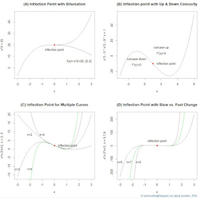
For a previous post on inflection points I needed a few examples, so I thought to write the code in the R language, which I did. Here's the final output:

Examples of Inflection Points

And, here's the code used to generate the above graphic:

par(mfrow = c(2,2)) #2x2 matrix display

# Example A: Inflection point with bifurcation
curve(x^3+20, -3,3, col = "black", main="(A) Inflection Point with Bifurcation")
curve(-x^2+20, 0, 3, add=TRUE, col="blue")
text (2, 10, "f(x)=-x^2+20, [0,3]", pos=1, offset = 1) #label inflection point
points(0, 20, col = "red", pch = 19) #inflection point 
text (0, 20, "inflection point", pos=1, offset = 1) #label inflection point


# Example B: Inflection point with Up & Down Concavity
curve(x^3-3*x^2-9*x+1, -3,6, main="(B) Inflection point with Up & Down Concavity")
points(1, -10, col = "red", pch = 19) #inflection point 
text (1, -10, "inflection point", pos=4, offset = 1) #label inflection point
text (-1, -10, "concave down", pos=3, offset = 1) 
text (-1, -10, "f''(x)<0", pos=1, offset = 0) 
text (2, 5, "concave up", pos=3, offset = 1)
text (2, 5, "f''(x)>0", pos=1, offset = 0) 


# Example C: Inflection point for multiple curves
curve(x^3-3*x+2, -3,3, col ="black", ylab="x^n-3*x+2, n = 2..5", main="(C) Inflection Point for Multiple Curves")
text (-3, -10, "n=3", pos=1) #label curve
curve(x^2-3*x+2,-3,3, add=TRUE, col="blue")
text (-2, 10, "n=2", pos=1) #label curve
curve(x^4-3*x+2,-3,3, add=TRUE, col="brown")
text (-1, 10, "n=4", pos=1) #label curve
curve(x^5-3*x+2,-3,3, add=TRUE, col="green")
text (-2, -10, "n=5", pos=1) #label curve
points(0, 2, col = "red", pch = 19) #inflection point 
text (0, 2, "inflection point", pos=4, offset = 1) #label inflection point
title("", line = -3, outer = TRUE)


# Example D: Inflection Point with fast change
curve(x^5-3*x+2,-3,3, col="black", ylab="x^n-3*x+2, n = 5,7,9", main="(D) Inflection Point with Slow vs. Fast Change")
text (-3, -100, "n=5", pos=1) #label curve
curve(x^7-3*x+2, add=TRUE, col="green")
text (-2.25, -100, "n=7", pos=1) #label curve
curve(x^9-3*x+2, add=TRUE, col="brown")
text (-1.5, -100, "n=9", pos=1) #label curve
points(0, 2, col = "red", pch = 19) #inflection point 
text (0, 2, "inflection point", pos=3, offset = 1) #label inflection point

mtext("© sql-troubles@blogspot.com @sql_troubles, 2024", side = 1, line = 4, adj = 1, col = "dodgerblue4", cex = .7)
#title("Examples of Inflection Points", line = -1, outer = TRUE)

Mathematically, an inflection point is a point on a smooth (plane) curve at which the curvature changes sign and where the second derivative is 0 [1]. The curvature intuitively measures the amount by which a curve deviates from being a straight line.

In example A, the main function has an inflection point, while the second function defined only for the interval [0,3] is used to represent a descending curve (aka bifurcation) for which the same point is a maximum point.  

In example B, the function was chosen to represent an example with a concave down (for which the second derivative is negative) and a concave up (for which the second derivative is positive) section. So what comes after an inflection point is not necessarily a monotonic increasing function. 

In example C are depicted several functions based on a varying power of the first coefficient which have the same inflection point. One could have shown only the behavior of the functions after the inflection point, while before choosing only one of the functions (see example A).

In example D is the same function as in example C with varying powers of the first coefficient considered, though for higher powers than in example C. I kept the function for n=5 to offer a basis for comparison. Apparently, the strange thing is that around the inflection point the change seems to be small and linear, which is not the case. The two graphics are correct though, because as basis is considered the scale for n=5, while in C the basis is n=3 (one scales the graphic further away from the inflection point). If one adds n=3 as the first function in the example D, the new chart will resemble C. Unfortunately, this behavior can be misused to show something like being linear around the inflection point, which is not the case. 

# Example E: Inflection Point with slow vs. fast change extended
curve(x^3-3*x+2,-3,3, col="black", ylab="x^n-3*x+2, n = 3,5,7,9", main="(E) Inflection Point with Slow vs. Fast Change")
text (-3, -10, "n=3", pos=1) #label curve
curve(x^5-3*x+2,-3,3, add=TRUE, col="brown")
text (-2, -10, "n=5", pos=1) #label curve
curve(x^7-3*x+2, add=TRUE, col="green")
text (-1.5, -10, "n=7", pos=1) #label curve
curve(x^9-3*x+2, add=TRUE, col="orange")
text (-1, -5, "n=9", pos=1) #label curve
points(0, 2, col = "red", pch = 19) #inflection point 
text (0, 2, "inflection point", pos=3, offset = 1) #label inflection point

Comments:
(1) I cheated a bit calculating the second derivative manually, which is an easy task for polynomials. There seems to be methods for calculating the inflection point, though the focus was on providing the examples. 
(2) The examples C and D could have been implemented as part of a loop, though I needed anyway to add the labels for each curve individually. Here's the modified code to support a loop:

# Example F: Inflection Point with slow vs. fast change with loop
n <- list(5,7,9)
color <- list("brown", "green", "orange")

curve(x^3-3*x+2,-3,3, col="black", ylab="x^n-3*x+2, n = 3,5,7,9", main="(F) Inflection Point with Slow vs. Fast Change")
for (i in seq_along(n))
{
ind <- as.numeric(n[i])
curve(x^ind-3*x+2,-3,3, add=TRUE, col=toString(color[i]))
}

text (-3, -10, "n=3", pos=1) #label curve
text (-2, -10, "n=5", pos=1) #label curve
text (-1, -5, "n=9", pos=1) #label curve
text (-1.5, -10, "n=7", pos=1) #label curve

Happy coding!

Previous Post <<||>> Next Post

References:
[1] Wikipedia (2023) Inflection point (link)

𖣯Strategic Management: Inflection Points and the Data Mesh (Quote of the Day)

Strategic Management Series

"Data mesh is what comes after an inflection point, shifting our approach, attitude, and technology toward data. Mathematically, an inflection point is a magic moment at which a curve stops bending one way and starts curving in the other direction. It’s a point that the old picture dissolves, giving way to a new one. [...] The impacts affect business agility, the ability to get value from data, and resilience to change. In the center is the inflection point, where we have a choice to make: to continue with our existing approach and, at best, reach a plateau of impact or take the data mesh approach with the promise of reaching new heights." [1]

I tried to understand the "metaphor" behind the quote. As the author through another quote pinpoints, the metaphor is borrowed from Andrew Groove:

"An inflection point occurs where the old strategic picture dissolves and gives way to the new, allowing the business to ascend to new heights. However, if you don’t navigate your way through an inflection point, you go through a peak and after the peak the business declines. [...] Put another way, a strategic inflection point is when the balance of forces shifts from the old structure, from the old ways of doing business and the old ways of competing, to the new. Before" [2]

The second part of the quote clarifies the role of the inflection point - the shift from a structure, respectively organization or system to a new one. The inflection point is not when we take a decision, but when the decision we took, and the impact shifts the balance. If the data mesh comes after the inflection point (see A), then there must be some kind of causality that converges uniquely toward the data mesh, which is questionable, if not illogical. A data mesh eventually makes sense after organizations reached a certain scale and thus is likely improbable to be adopted by small to medium businesses. Even for large organizations the data mesh may not be a viable solution if it doesn't have a proven record of success. 

I could understand if the author would have said that the data mesh will lead to an inflection point after its adoption, as is the case of transformative/disruptive technologies. Unfortunately, the tracking record of BI and Data Analytics projects doesn't give many hopes for such a magical moment to happen. Probably, becoming a data-driven organization could have such an effect, though for many organizations the effects are still far from expectations. 

There's another point to consider. A curve with inflection points can contain up and down concavities (see B) or there can be multiple curves passing through an inflection point (see C) and the continuation can be on any of the curves.

Examples of Inflection Points [3]

The change can be fast or slow (see D), and in the latter it may take a long time for change to be perceived. Also [2] notes that the perception that something changed can happen in stages. Moreover, the inflection point can be only local and doesn't describe the future evolution of the curve, which to say that the curve can change the trajectory shortly after that. It happens in business processes and policy implementations that after a change was made in extremis to alleviate an issue a slight improvement is recognized after which the performance decays sharply. It's the case of situations in which the symptoms and not the root causes were addressed. 

More appropriate to describe the change would be a tipping point, which can be defined as a critical threshold beyond which a system (the organization) reorganizes/changes, often abruptly and/or irreversible.

Previous Post <<||>> Next Post

References:
[1] Zhamak Dehghani (2021) Data Mesh: Delivering Data-Driven Value at Scale (book review)
[2] Andrew S Grove (1988) "Only the Paranoid Survive: How to Exploit the Crisis Points that Challenge Every Company and Career"
[3] SQL Troubles (2024) R Language: Drawing Function Plots (Part II - Basic Curves & Inflection Points) (link)

♟️Strategic Management: Strategy (Notes)

Disclaimer: This is work in progress intended to consolidate information from various sources. 
Last updated: 18-Mar-2024

Strategy

• {definition} "the determination of the long-term goals and objectives of an enterprise, and the adoption of courses of action and the allocation of resources necessary for carrying out these goals" [4]
• {goal} bring all tools and insights together to create an integrative narrative about what the  organization should do moving forward [1]
• a good strategy emerges out of the values, opportunities and capabilities of the organization [1]
• {characteristic} robust
• {characteristic} flexible
• {characteristic} needs to embrace the uncertainty and complexity of the world
• {characteristic} fact-based and informed by research and analytics
• {characteristic} testable
• {concept} strategy analysis 
• {definition} the assessment of an organization's current competitive position and the identification of future valuable competitive positions and how the firm plans to achieve them [1]
• done from a general perspective
• in terms of different functional elements within the organization [1]
• in terms of being integrated across different concepts and tools and frameworks [1]
• a good strategic analysis integrates various tools and frameworks that are in our strategist toolkit [1]
• approachable in terms of 
• dynamics
• complexity
• competition
• {step} identify the mission and values of the organization
• critical for understanding what the firm values and how it may influence where opportunities they look for and what actions they might be willing to take
• {step} analyze the competitive environment
• looking at what opportunities the environment provides, how are competitors likely to react
• {step} analyze competitive positions
• think about  own capabilities are and how they might relate to the opportunities that are available
• {step} analyze and recommend strategic actions 
• actions for future improvement
• {question} how do we create more value?
• {question} how can we improve our current competitive position?
• {question} how can we in essence, create more value in our competitive environment
• alternatives
• scaling the business
• entering new markets
• innovating
• acquiring a competitor/another player within a market segment of interest
• recommendations
• {question} what do we recommend doing going forward?
• {question} what are the underlying assumptions of these recommendations?
• {question} do they meet our tests that we might have for providing value?
• move from analysis to action
• actions come from asking a series of questions about what opportunities, what actions can we take moving forward
• {step} strategy formulation
• {step} strategy implementation
• {tool} competitor analysis
• {question} what market is the firm in, and who are the players in these markets? 
• {tool} environmental analysis
• {benefit} provides a picture on the broader competitive environment
• {question} what are the major trends impacting this industry?
• {question} are there changes in the sociopolitical environment that are going to have important implications for this industry?
• {question} is this an attractive market or the barrier to competition?
• {tool} five forces analysis
• {benefit} provides an overview of the market structure/industry structure
• {benefit} helps understand the nature of the competitive game that we are playing as we then devise future strategies [1]
• provides a dynamic perspective in our understanding of a competitive market
• {question} how's the competitive structure in a market likely to evolve?
• {tool} competitive lifestyle analysis
• {tool} SWOT (strengths, weaknesses, opportunities, threats) analysis
• {tool} stakeholder analysis
• {benefit} valuable in trying to understand those mission and values and then the others expectations of a firm
• {tool} capabilities analysis
• {question} what are the firm's unique resources and capabilities?
• {question} how sustainable as any advantage that these assets provide?
• {tool} portfolio planning matrix
• {benefit} helps us now understand how they might leverage these assets across markets, so as to improve their position in any given market here
• {question} how should we position ourselves in the market relative to our rivals?
• {tool} capability analysis
• {benefit} understand what the firm does well and see what opportunities they might ultimately want to attack and go after in terms of these valuable competitive positions
• via Strategy Maps and Portfolio Planning matrices
• {tool} hypothesis testing
• {question} how competitors are likely to react to these actions?
• {question} does it make sense in the future worlds we envision?
• [game theory] pay off matrices can be useful to understand what actions taken by various competitors within an industry
• {tool} scenario planning
• {benefit} helps us envision future scenarios and then work back to understand what are the actions we might need to take in those various scenarios if they play out.
• {question} does it provide strategic flexibility?
• {tool} real options analysis 
• highlights the desire to have strategic flexibility or at least the value of strategic flexibility provides
• {tool} acquisition analysis
• {benefit} helps understand the value of certain action versus others
• {benefit} useful as an understanding of opportunity costs for other strategic investments one might make
• focused on mergers and acquisitions
• {tool} If-Then thinking
• sequential in nature
• different from causal logic
• commonly used in network diagrams, flow charts, Gannt charts, and computer programming
• {tool} Balanced Scorecard
• {definition} a framework to look at the strategy used for value creation from four different perspectives [5]
• {perspective} financial 
• {scope} the strategy for growth, profitability, and risk viewed from the perspective of the shareholder [5]
• {question} what are the financial objectives for growth and productivity? [5]
• {question} what are the major sources of growth? [5]
• {question} If we succeed, how will we look to our shareholders? [5]
• {perspective} customer
• {scope} the strategy for creating value and differentiation from the perspective of the customer [5]
• {question} who are the target customers that will generate revenue growth and a more profitable mix of products and services? [5]
• {question} what are their objectives, and how do we measure success with them? [5]
• {perspective} internal business processes
• {scope} the strategic priorities for various business processes, which create customer and shareholder satisfaction [5] 
• {perspective} learning and growth 
• {scope} defines the skills, technologies, and corporate culture needed to support the strategy. 
• enable a company to align its human resources and IT with its strategy
• {benefit} enables the strategic hypotheses to be described as a set of cause-and-effect relationships that are explicit and testable [5]
• require identifying the activities that are the drivers (or lead indicators) of the desired outcomes (lag indicators)  [5]
• everyone in the organization must clearly understand the underlying hypotheses, to align resources with the hypotheses, to test the hypotheses continually, and to adapt as required in real time [5]
• {tool} strategy map
• {definition} a visual representation of a company’s critical objectives and the crucial relationships that drive organizational performance [2]
• shows the cause-and effect links by which specific improvements create desired outcomes [2]
• {benefit} shows how an organization will convert its initiatives and resources–including intangible assets such as corporate culture and employee knowledge into tangible outcomes [2]
• {component} mission
• {question} why we exist?
• {component} core values
• {question} what we believe in?
• ⇐ mission and the core values  remain fairly stable over time [5]
• {component} vision
• {question} what we want to be?
• paints a picture of the future that clarifies the direction of the organization [5]
• helps-individuals to understand why and how they should support the organization [5]

Previous Post <<||>> Next Post

References:
[1] University of Virginia (2022) Strategic Planning and Execution (MOOC, Coursera)
[2] Robert S Kaplan & David P Norton (2000) Having Trouble with Your Strategy? Then Map It (link)
[3] Harold Kerzner (2001) Strategic planning for project management using a project management maturity model
[4] Alfred D Chandler Jr. (1962) "Strategy and Structure"
[5] Robert S Kaplan & David P Norton (2000) The Strategy-focused Organization: How Balanced Scorecard Companies Thrive in the New Business Environment

🧭Business Intelligence: Data Products (Part II: The Complexity Challenge)

Business Intelligence Series

Creating data products within a data mesh resumes in "partitioning" a given set of inputs, outputs and transformations to create something that looks like a Lego structure, in which each Lego piece represents a data product. The word partition is improperly used as there can be overlapping in terms of inputs, outputs and transformations, though in an ideal solution the outcome should be close to a partition.

If the complexity of inputs and outputs can be neglected, even if their number could amount to a big number, not the same can be said about the transformations that must be performed in the process. Moreover, the transformations involve reengineering the logic built in the source systems, which is not a trivial task and must involve adequate testing. The transformations are a must and there's no way to avoid them. 

When designing a data warehouse or data mart one of the goals is to keep the redundancy of the transformations and of the intermediary results to a minimum to minimize the unnecessary duplication of code and data. Code duplication becomes usually an issue when the logic needs to be changed, and in business contexts that can happen often enough to create other challenges. Data duplication becomes an issue when they are not in synch, fact derived from code not synchronized or with different refresh rates.

Building the transformations as SQL-based database objects has its advantages. There were many attempts for providing non-SQL operators for the same (in SSIS, Power Query) though the solutions built based on them are difficult to troubleshoot and maintain, the overall complexity increasing with the volume of transformations that must be performed. In data mashes, the complexity increases also with the number of data products involved, especially when there are multiple stakeholders and different goals involved (see the challenges for developing data marts supposed to be domain-specific). 

To growing complexity organizations answer with complexity. On one side the teams of developers, business users and other members of the governance teams who together with the solution create an ecosystem. On the other side, the inherent coordination and organization meetings, managing proposals, the negotiation of scope for data products, their design, testing, etc.  The more complex the whole ecosystem becomes, the higher the chances for systemic errors to occur and multiply, respectively to create unwanted behavior of the parties involved. Ecosystems are challenging to monitor and manage. 

The more complex the architecture, the higher the chances for failure. Even if some organizations might succeed, it doesn't mean that such an endeavor is for everybody - a certain maturity in building data architectures, data-based artefacts and managing projects must exist in the organization. Many organizations fail in addressing basic analytical requirements, why would one think that they are capable of handling an increased complexity? Even if one breaks the complexity of a data warehouse to more manageable units, the complexity is just moved at other levels that are more difficult to manage in ensemble. 

Being able to audit and test each data product individually has its advantages, though when a data product becomes part of an aggregate it can be easily get lost in the bigger picture. Thus, is needed a global observability framework that allows to monitor the performance and health of each data product in aggregate. Besides that, there are needed event brokers and other mechanisms to handle failure, availability, security, etc. 

Data products make sense in certain scenarios, especially when the complexity of architectures is manageable, though attempting to redesign everything from their perspective is like having a hammer in one's hand and treating everything like a nail.

Previous Post <<||>> Next Post

🧭Business Intelligence: Data Products (Part I: A Lego Exercise)

Business Intelligence Series

One can define a data product as the smallest unit of data-driven architecture that can be independently deployed and managed (aka product quantum) [1]. In other terms one can think of a data product like a box (or Lego piece) which takes data as inputs, performs several transformations on the data from which result several output data (or even data visualizations or a hybrid between data, visualizations and other content). 

At high-level each Data Analytics solution can be regarded as a set of inputs, a set of outputs and the transformations that must be performed on the inputs to generate the outputs. The inputs are the data from the operational systems, while the outputs are analytics data that can be anything from data to KPIs and other metrics. A data mart, data warehouse, lakehouse and data mesh can be abstracted in this way, though different scales apply. 

For creating data products within a data mesh, given a set of inputs, outputs and transformations, the challenge is to find horizontal and vertical partitions within these areas to create something that looks like a Lego structure, in which each piece of Lego represents a data product, while its color represents the membership to a business domain. Each such piece is self-contained and contains a set of transformations, respectively intermediary inputs and outputs. Multiple such pieces can be combined in a linear or hierarchical fashion to transform the initial inputs into the final outputs. 

Data Products with a Data Mesh

Finding such a partition is possible though it involves a considerable effort, especially in designing the whole thing - identifying each Lego piece uniquely. When each department is on its own and develops its own Lego pieces, there's no guarantee that the pieces from the various domains will fit together to built something cohesive, performant, secure or well-structured. Is like building a house from modules, the pieces must fit together. That would be the role of governance (federated computational governance) - to align and coordinate the effort. 

Conversely, there are transformations that need to be replicated for obtaining autonomous data products, and the volume of such overlapping can be considerable high. Consider for example the logic available in reports and how often it needs to be replicated. Alternatively, one can create intermediary data products, when that's feasible. 

It's challenging to define the inputs and outputs for a Lego piece. Now imagine in doing the same for a whole set of such pieces depending on each other! This might work for small pieces of data and entities quite stable in their lifetime (e.g. playlists, artists, songs), but with complex information systems the effort can increase by a few factors. Moreover, the complexity of the structure increases as soon the Lego pieces expand beyond their initial design. It's like the real Lego pieces would grow within the available space but still keep the initial structure - strange constructs may result, which even if they work, change the gravity center of the edifice in other directions. There will be thus limits to grow that can easily lead to duplication of functionality to overcome such challenges.

Each new output or change in the initial input for this magic boxes involves a change of all the intermediary Lego pieces from input to output. Just recollect the last experience of defining the inputs and the outputs for an important complex report, how many iterations and how much effort was involved. This might have been an extreme case, though how realistic is the assumption that with data products everything will go smoother? No matter of the effort involved in design, there will be always changes and further iterations involved.

Previous Post <<||>> Next Post

References:
[1] Zhamak Dehghani (2021) Data Mesh: Delivering Data-Driven Value at Scale (book review) 

🧭Business Intelligence: A Software Engineer's Perspective (Part VII: Think for Yourself!)

Business Intelligence Series

After almost a quarter-century of professional experience the best advice I could give to younger professionals is to "gather information and think for themselves", and with this the reader can close the page and move forward! Anyway, everybody seems to be looking for sudden enlightenment with minimal effort, as if the effort has no meaning in the process!

In whatever endeavor you are caught, it makes sense to do upfront a bit of thinking for yourself - what's the task, or more general the problem, which are the main aspects and interpretations, which are the goals, respectively the objectives, how a solution might look like, respectively how can it be solved, how long it could take, etc. This exercise is important for familiarizing yourself with the problem and creating a skeleton on which you can build further. It can be just vague ideas or something more complex, though no matter the overall depth is important to do some thinking for yourself!

Then, you should do some research to identify how others approached and maybe solved the problem, what were the justifications, assumptions, heuristics, strategies, and other tools used in sense-making and problem solving. When doing research, one should not stop with the first answer and go with it. It makes sense to allocate a fair amount of time for information gathering, structuring the findings in a reusable way (e.g. tables, mind maps or other tools used for knowledge mapping), and looking at the problem from the multiple perspectives derived from them. It's important to gather several perspectives, otherwise the decisions have a high chance of being biased. Just because others preferred a certain approach, it doesn't mean one should follow it, at least not blindly!

The purpose of research is multifold. First, one should try not to reinvent the wheel. I know, it can be fun, and a lot can be learned in the process, though when time is an important commodity, it's important to be pragmatic! Secondly, new information can provide new perspectives - one can learn a lot from other people’s thinking. The pragmatism of problem solvers should be combined, when possible, with the idealism of theories. Thus, one can make connections between ideas that aren't connected at first sight.

Once a good share of facts was gathered, you can review the new information in respect to the previous ones and devise from there several approaches worthy of attack. Once the facts are reviewed, there are probably strong arguments made by others to follow one approach over the others. However, one can show that has reached a maturity when is able to evaluate the information and take a decision based on the respective information, even if the decision is not by far perfect.

One should try to develop a feeling for decision making, even if this seems to be more of a gut-feeling and stressful at times. When possible, one should attempt to collect and/or use data, though collecting data is often a luxury that tends to postpone the decision making, respectively be misused by people just to confirm their biases. Conversely, if there's any important benefit associated with it, one can collect data to validate in time one's decision, though that's a more of a scientist’s approach.

I know that's easier to go with the general opinion and do what others advise, especially when some ideas are popular and/or come from experts, though then would mean to also follow others' mistakes and biases. Occasionally, that can be acceptable, especially when the impact is neglectable, however each decision we are confronted with is an opportunity to learn something, to make a difference! 

Previous Post <<||>> Next Post

🧊🗒️Data Warehousing: Data Mesh (Notes)

Disclaimer: This is work in progress intended to consolidate information from various sources. 
Last updated: 17-Mar-2024

Data Products with a Data Mesh

Data Mesh

• {definition} "a sociotechnical approach to share, access and manage analytical data in complex and large-scale environments - within or across organizations" [1]
• ⇐ there is no default standard or reference implementation of data mesh and its components [2]
• {definition} a type of decentralized data architecture that organizes data based on different business domains [2]
• ⇐ no centralized data architecture coexists with data mesh, unless in transition [1]
• distributes the modeling of analytical data, the data itself and its ownership [1]
• {characteristic} partitions data around business domains and gives data ownership to the domains [1]
• each domain can model their data according to their context [1]
• there can be multiple models of the same concept in different domains gives the data sharing responsibility to those who are most intimately familiar with the data [1]
• endorses multiple models of the data
• data can be read from one domain, transformed and stored by another domain [1]
• {characteristic} evolutionary execution process
• {characteristic} agnostic of the underlying technology and infrastructure [1]
• {aim} respond gracefully to change [1]
• {aim} sustain agility in the face of growth [1]
• {aim} increase the ratio of value from data to investment [1]
• {principle} data as a product
• {goal} business domains become accountable to share their data as a product to data users
• {goal} introduce a new unit of logical architecture that controls and encapsulates all the structural components needed to share data as a product autonomously [1]
• {goal} adhere to a set of acceptance criteria that assure the usability, quality, understandability, accessibility and interoperability of data products*
• usability characteristics
• {principle} domain-oriented ownership
• {goal} decentralize the ownership of sharing analytical data to business domains that are closest to the data [1]
• {goal} decompose logically the data artefacts based on the business domain they represent and manage their life cycle independently [1]
• {goal} align business, technology and analytical data [1]
• {principle} self-serve data platform
• {goal} provide a self-serve data platform to empower domain-oriented teams to manage and govern the end-to-end life cycle of their data products* [1]
• {goal} streamline the experience of data consumers to discover, access, and use the data products [1]
• {principle} federated computational governance
• {goal} implement a federated decision making and accountability structure that balances the autonomy and agility of domains, while respecting the global conformance, interoperability and security of the mesh* [1]
• {goal} codifying and automated execution of policies at a fine-grained level [1]
• ⇐ the principles represent a generalization and adaptation of practices that address the scale of organization digitization* [1]
• {concept} decentralization of data products
• {requirement} ability to compose data across different modes of access and topologies [1]
• data needs to be agnostic to the syntax of data, underlying storage type, and mode of access to it [1]
• many of the existing composability techniques that assume homogeneous data won’t work
• e.g.  defining primary and foreign key relationships between tables of a single schema [1]
• {requirement} ability to discover and learn what is relatable and decentral [1]
• {requirement} ability to seamlessly link relatable data [1]
• {requirement} ability to relate data temporally [1]
• {concept} data product 
• the smallest unit of data-based architecture that can be independently deployed and managed (aka product quantum) [1]
• provides a set of explicitly defined and data sharing contracts
• provides a truthful portion of the reality for a particular domain (aka single slice of truth) [1]
• constructed in alignment with the source domain [3]
• {characteristic} autonomous
• its life cycle and model are managed independently of other data products [1]
• {characteristic} discoverable
• via a centralized registry or catalog that list the available datasets with some additional information about each dataset, the owners, the location, sample data, etc. [1]
• {characteristic} addressable
• via a permanent and unique address to the data user to programmatically or manually access it [1] 
• {characteristic} understandable
• involves getting to know the semantics of its underlying data and the syntax in which the data is encoded [1]
• describes which entities it encapsulates, the relationships between them, and their adjacent data products [1]
• {characteristic} trustworthy and truthful
• represents the fact of the business correctly [1]
• provides data provenance and data lineage [1]
• {characteristic} natively accessible
• make it possible for various data users to access and read its data in their native mode of access [1]
• meant to be broadcast and shared widely [3]
• {characteristic} interoperable and composable
• follows a set of standards and harmonization rules that allow linking data across domains easily [1]
• {characteristic} valuable on its own
• must have some inherent value for the data users [1]
• {characteristic} secure
• the access control is validated by the data product, right in the flow of data, access, read, or write [1] 
• ⇐ the access control policies can change dynamically
• {characteristic} multimodal 
• there is no definitive 'right way' to create a data product, nor is there a single expected form, format, or mode that it is expected to take [3] 
• shares its logs, traces, and metrics while consuming, transforming, and sharing data [1]
• {concept} data quantum (aka product data quantum, architectural quantum) 
• unit of logical architecture that controls and encapsulates all the structural components needed to share a data product [1]
• {component} data
• {component} metadata
• {component} code
• {component} policies
• {component} dependencies' listing
• {concept} data product observability
• monitor the operational health of the mesh
• debug and perform postmortem analysis
• perform audits
• understand data lineage
• {concept} logs 
• immutable, timestamped, and often structured events that are produced as a result of processing and the execution of a particular task [1]
• used for debugging and root cause analysis
• {concept} traces
• records of causally related distributed events [1]
• {concept} metrics
• objectively quantifiable parameters that continue to communicate build-time and runtime characteristics of data products [1]
• artefacts 
• e.g. data, code, metadata, policies

References:
[1] Zhamak Dehghani (2021) Data Mesh: Delivering Data-Driven Value at Scale (book review)
[2] Zhamak Dehghani (2019) How to Move Beyond a Monolithic Data Lake to a Distributed Data Mesh (link)
[3] Adam Bellemare (2023) Building an Event-Driven Data Mesh: Patterns for Designing and Building Event-Driven Architectures

🧭Business Intelligence: Architecture (Part I: Monolithic vs. Distributed and Zhamak Dehghani's Data Mesh - Debunked)

Business Intelligence Series

In [1] the author categorizes data warehouses (DWHs) and lakes as monolithic architectures, as opposed to data mesh's distributed architecture, which makes me circumspect about term's use. There are two general definitions of what monolithic means: (1) formed of a single large block (2) large, indivisible, and slow to change.

In software architecture one can differentiate between monolithic applications where the whole application is one block of code, multi-tier applications where the logic is split over several components with different functions that may reside on the same machine or are split non-redundantly between multiple machines, respectively distributed, where the application or its components run on multiple machines in parallel.

Distributed multi-tire applications are a natural evolution of the two types of applications, allowing to distribute redundantly components across multiple machines. Much later came the cloud where components are mostly entirely distributed within same or across distinct geo-locations, respectively cloud providers.

Data Warehouse vs. Data Lake vs. Lakehouse [2]

From licensing and maintenance convenience, a DWH resides typically on one powerful machine with many chores, though components can be moved to other machines and even distributed, the ETL functionality being probably the best candidate for this. In what concerns the overall schema there can be two or more data stores with different purposes (operational/transactional data stores, data marts), each of them with their own schema. Each such data store could be moved on its own machine though that's not feasible.

DWHs tend to be large because they need to accommodate a considerable number of tables where data is extracted, transformed, and maybe dumped for the various needs. With the proper design, also DWHs can be partitioned in domains (e.g. define one schema for each domain) and model domain-based perspectives, at least from a data consumer's perspective. The advantage a DWH offers is that one can create general dimensions and fact tables and build on top of them the domain-based perspectives, minimizing thus code's redundancy and reducing the costs.  

With this type of design, the DWH can be changed when needed, however there are several aspects to consider. First, it takes time until the development team can process the request, and this depends on the workload and priorities set. Secondly, implementing the changes should take a fair amount of time no matter of the overall architecture used, given that the transformations that need to be done on the data are largely the same. Therefore, one should not confuse the speed with which a team can start working on a change with the actual implementation of the change. Third, the possibility of reusing existing objects can speed up changes' implementation. 

Data lakes are distributed data repositories in which structured, unstructured and semi-structured data are dumped in raw form in standard file formats from the various sources and further prepared for consumption in other data files via data pipelines, notebooks and similar means. One can use the medallion architecture with a folder structure and adequate permissions for domains and build reports and other data artefacts on top. 

A data lake's value increases when is combined with the capabilities of a DWH (see dedicated SQL server pool) and/or analytics engine (see serverless SQL pool) that allow(s) building an enterprise semantic model on top of the data lake. The result is a data lakehouse that from data consumer's perspective and other aspects mentioned above is not much different than the DWH. The resulting architecture is distributed too. 

Especially in the context of cloud computing, referring to nowadays applications metaphorically (for advocative purposes) as monolithic or distributed is at most a matter of degree and not of distinction. Therefore, the reader should be careful!

Previous Post <<||>> Next Post

References:
[1] Zhamak Dehghani (2021) Data Mesh: Delivering Data-Driven Value at Scale (book review)
[2] Databricks (2022) Data Lakehouse (link)

🔖Book Review: Zhamak Dehghani's Data Mesh: Delivering Data-Driven Value at Scale (2021)

	Zhamak Dehghani's "Data Mesh: Delivering Data-Driven Value at Scale" (2021) is a must read book for the data professional. So, here I am, finally managing to read it and give it some thought, even if it will probably take more time and a few more reads for the ideas to grow. Working in the fields of Business Intelligence and Software Engineering for almost a quarter-century, I think I can understand the historical background and the direction of the ideas presented in the book. There are many good ideas but also formulations that make me circumspect about the applicability of some assumptions and requirements considered.  So, after data marts, warehouses, lakes and lakehouses, the data mesh paradigm seems to be the new shiny thing that will bring organizations beyond the inflection point with tipping potential from where organization's growth will have an exponential effect. At least this seems to be the first impression when reading the first chapters.
The book follows to some degree the advocative tone of promoting that "our shiny thing is much better than previous thing", or "how bad the previous architectures or paradigms were and how good the new ones are" (see [2]). Architectures and paradigms evolve with the available technologies and our perception of what is important for businesses. Old and new have their place in the order of things, and the old will continue to exist, at least until the new proves its feasibility.   The definition of the data mash as "a sociotechnical approach to share, access and manage analytical data in complex and large-scale environments - within or across organizations" [1] is too abstract even if it reflects at high level what the concept is about. Compared to other material I read on the topic, the book succeeds in explaining the related concepts as well the goals (called definitions) and benefits (called motivations) associated with the principles behind the data mesh, making the book approachable also by non-professionals.  Built around four principles "data as a product", "domain-oriented ownership", "self-serve data platform" and "federated governance", the data mesh is the paradigm on which data as products are developed; where the products are "the smallest unit of architecture that can be independently deployed and managed", providing by design the information necessary to be discovered, understood, debugged, and audited. It's possible to create Lego-like data products, data contracts and/or manifests that address product's usability characteristics, though unless the latter are generated automatically, put in the context of ERP and other complex systems, everything becomes quite an endeavor that requires time and adequate testing, increasing the overall timeframe until a data product becomes available.  The data mesh describes data products in terms of microservices that structure architectures in terms of a collection of services that are independently deployable and loosely coupled. Asking from data products to behave in this way is probably too hard a constraint, given the complexity and interdependency of the data models behind business processes and their needs. Does all the effort make sense? Is this the "agility" the data mesh solutions are looking for? Many pioneering organizations are still fighting with the concept of data mesh as it proves to be challenging to implement. At a high level everything makes sense, but the way data products are expected to function makes the concept challenging to implement to the full extent. Moreover, as occasionally implied, the data mesh is about scaling data analytics solutions with the size and complexity of organizations. The effort makes sense when the organizations have a certain size and the departments have a certain autonomy, therefore, it might not apply to small to medium businesses. Previous Post <<||>>  Next Post References: [1] Zhamak Dehghani (2021) "Data Mesh: Delivering Data-Driven Value at Scale" (link) [2] SQL-troubles (2024) Zhamak Dehghani's Data Mesh - Monolithic Warehouses and Lakes (link)